Estimated inundation time by CCHA transect

library(tidyverse)
library(cobs)
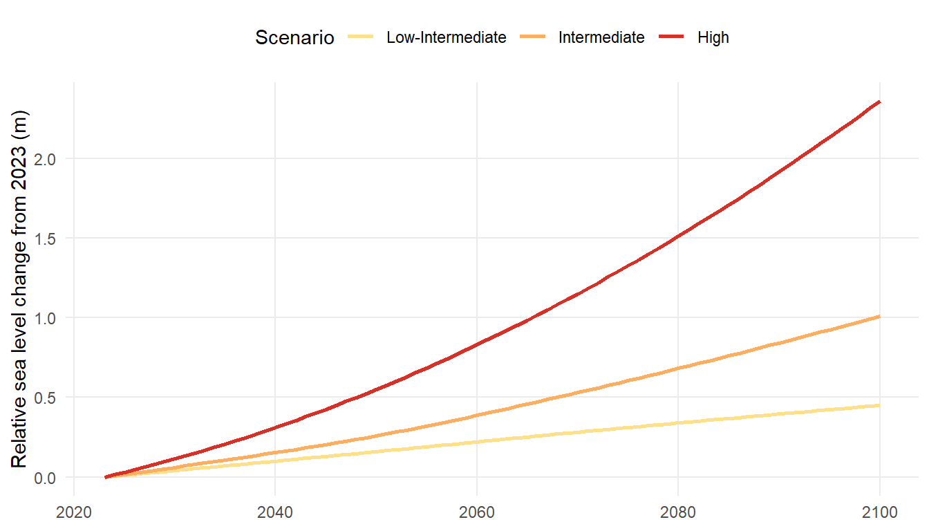
library(here)

This analysis is a potential inundation scenario for the CCHA transects based on sea level rise projections in the Tampa Bay region. Sea level is based on the St. Petersburg NOAA tide guage (8726520) and three scenarios of low-intermediate, intermediate, and high projection estimates consistent with the National Climate Assessment (as described in TBEP technical publication #05-19). Zero accretion and no inland migration of habitats is assumed and estimates herein are conservative. The 2023 sea level is the recorded elevation at the start of each transect.

# msl2023 <- read.table('https://tidesandcurrents.noaa.gov/sltrends/data/8726520_meantrend.csv', sep = ',',
#                   skip = 6, header = F) %>% 
#   select(
#     Year = V1, 
#     Month = V2, 
#     MSL = V3
#   ) %>% 
#   mutate(
#     Date = lubridate::make_date(Year, Month, 1)
#   ) %>% 
#   filter(Year == 2023) %>% 
#   pull(MSL) %>%
#   mean() 

# scnario colors as ramp
scencols <- c( '#fee08b', '#fdae61', '#d73027')

# from TBEP #05-19   
scen <- tibble::tribble(
    ~yrs, ~low, ~mid, ~high,
    2000,  0,    0,    0,
    2030,  0.56, 0.79, 1.25,
    2040,  0.72, 1.08, 1.77,
    2050,  0.95, 1.44, 2.56,
    2060,  1.15, 1.87, 3.48,
    2070,  1.35, 2.33, 4.56,
    2080,  1.54, 2.82, 5.71,
    2090,  1.71, 3.38, 7.05,
    2100,  1.90, 3.90, 8.50
  )

# interpolate tidal increase each year using a spline with constant rate increase
yrest <- 2000:2100
scenapprox <- scen %>% 
  pivot_longer(names_to = 'scenario', values_to = 'feet', -yrs) %>% 
  mutate(
    scenario = factor(scenario, levels = c('low', 'mid', 'high'), 
                      labels = c('Low-Intermediate', 'Intermediate', 'High')
    )
  ) %>% 
  group_nest(scenario) %>% 
  mutate(
    pred = purrr::map(data, function(data){
      
      cobs_fit <- cobs(data$yrs, data$feet, constraint = "increase", nknots = 5, print.mesg = F, print.warn = F)
      cobs_pred <- predict(cobs_fit, nz = length(yrest))

      tibble(
        yrs = yrest, 
        feet = cobs_pred[,2]
      )
  
    })
  ) %>% 
  select(-data) %>% 
  unnest('pred') %>% 
  mutate(
    MSL_m = feet * 0.3048
  ) %>%  
  filter(yrs >= 2023) %>% 
  mutate(
    chg_m = c(0, diff(MSL_m)), 
    MSL_m = cumsum(chg_m),
    .by = scenario
  ) %>% 
  # mutate(
  #   MSL_m = chg_m + msl2023,
  # ) %>% 
  select(scenario, yrs, MSL_m) #%>%
  # group_nest(yrs, .key = 'MSL_m')

ggplot(scenapprox, aes(x = yrs, y = MSL_m, color = scenario)) + 
  theme_minimal() + 
  theme(
    panel.grid.minor = element_blank(), 
    legend.position = 'top'
  ) +
  scale_color_manual(values = scencols) + 
  geom_line(linewidth = 1) + 
  labs(
    x = NULL, 
    y = 'Relative sea level change from 2023 (m)', 
    color = 'Scenario'
  )

Relative sea level change from 2023 for three scenarios of sea level rise in the Tampa Bay region.

vegdatele <- read.csv(here('data/raw/vegdatele.csv'))

# starting elevation
strele <- vegdatele %>% 
  filter(Sample_set == 3) %>% 
  select(Site, Meter, Elevation_NAVD88) %>% 
  distinct() %>% 
  filter(Meter == 0) %>% 
  select(-Meter)

scenapproxsite <- crossing(strele, scenapprox) %>% 
  mutate(MSL_m = MSL_m + Elevation_NAVD88) %>% 
  select(-Elevation_NAVD88)

# # accretion rates, based on RTK elevation diff per year  
# accrt <- vegdatele %>%
#   mutate(
#     yr = year(mdy(Date))
#   ) %>% 
#   summarise(
#     meanele = mean(Elevation_NAVD88, na.rm = T), 
#     .by = c(Site, yr)
#   ) %>% 
#   summarise(
#     elediff = diff(meanele), 
#     yrdiff = diff(yr), 
#     .by = Site
#   ) %>% 
#   mutate(
#     accrate = elediff / yrdiff
#   ) %>% 
#   select(Site, accrate)

ele <- vegdatele %>% 
  filter(Sample_set == 3) %>% 
  select(Site, Simplified_zone_name, Meter, Elevation_NAVD88) %>% 
  distinct() %>% 
  group_nest(Site) %>% 
  crossing(
    yrs = 2023:2100 
  )

# join data for eval
jndat <- ele %>% #full_join(ele, accrt, by = 'Site') %>% 
  full_join(scenapproxsite, by = c('yrs', 'Site'), relationship = 'many-to-many') %>% 
  # mutate(
  #   acc = c(0, cumsum(accrate[-1])),
  #   .by = Site
  # ) %>% 
  # select(-accrate) %>% 
  # mutate(
  #   data = purrr::pmap(list(acc, data), function(acc, data){
  #     
  #     data %>%
  #       mutate(
  #         Elevation_NAVD88 = Elevation_NAVD88 + acc
  #       )
  # 
  #   })
  # ) %>% 
  # select(-acc) %>% 
  unnest(data)

# percent inundated over time (assumes no accretion)
inund <- jndat %>% 
  summarise(
    perinund = sum(Elevation_NAVD88 < MSL_m) / n(),
    .by = c(Site, yrs, scenario)
  ) 

# percent zone inundation over time (assumes no accretion)
zoneinund <- jndat %>% 
  summarise(
    perinund = sum(Elevation_NAVD88 < MSL_m) / n(),
    .by = c(Simplified_zone_name, yrs, scenario)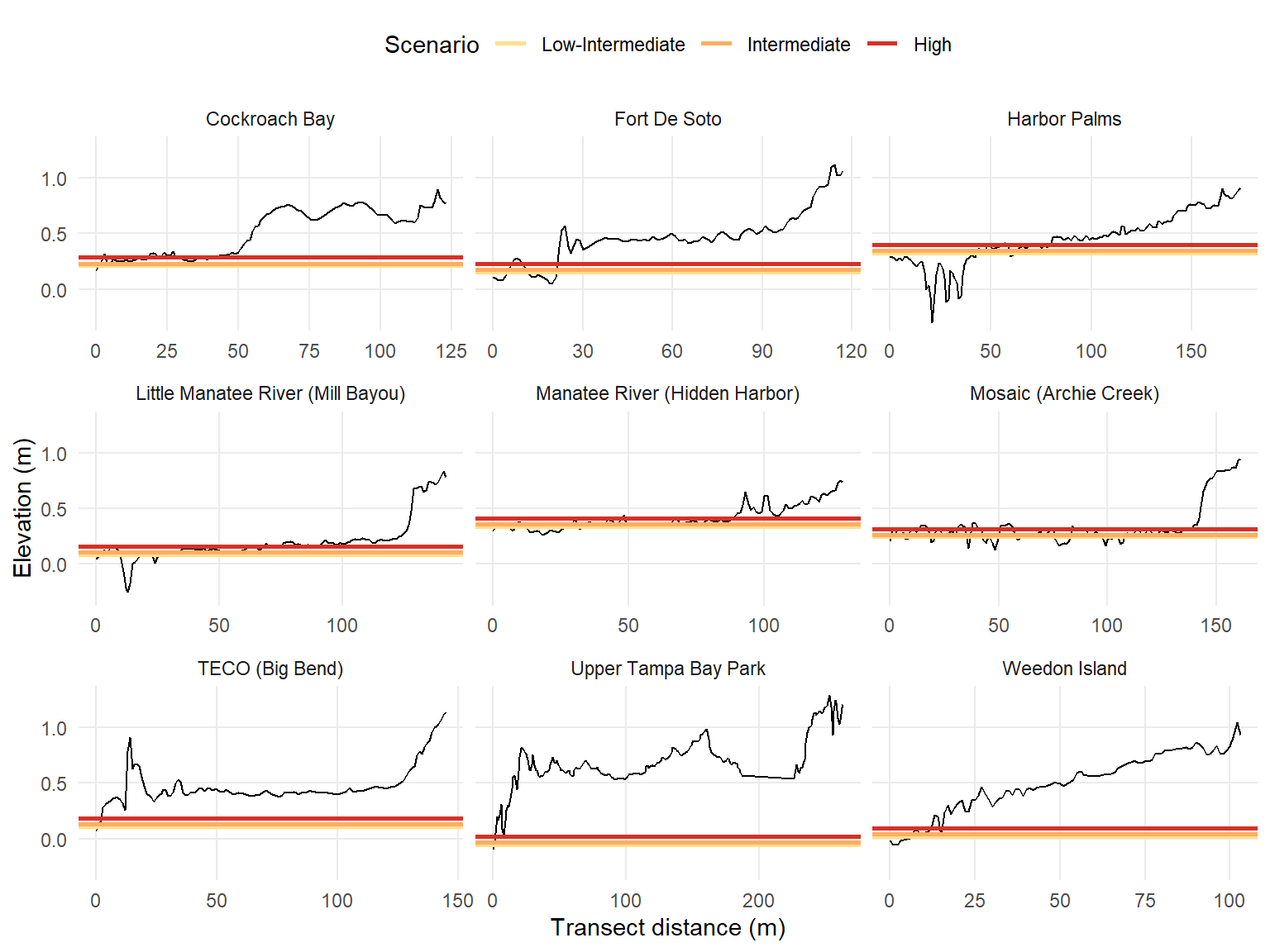
  ) 

2030 - HMP targets

toplo1 <- jndat %>% 
  filter(yrs %in% c(2030))

ggplot(toplo1, aes(x = Meter, y = Elevation_NAVD88)) + 
  geom_line() +
  facet_wrap(~Site, scales = 'free_x') +
  geom_hline(aes(yintercept = MSL_m, color = scenario), linewidth = 1) +
  scale_color_manual(values = scencols) +
  theme_minimal() +
  theme(
    panel.grid.minor = element_blank(),
    legend.position = 'top'
  ) + 
  labs(
    x = 'Transect distance (m)',
    y = 'Elevation (m)',
    color = 'Scenario'
  )

Projected relative sea level rise in 2030 for three scenarios by CCHA transect. Assumes no accretion nor inland migration.

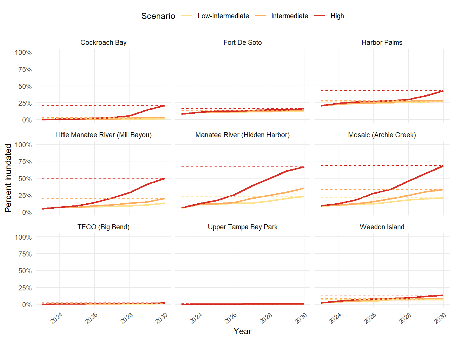
maxyr <- 2030
toplo2 <- inund %>% 
  filter(yrs <= maxyr)
perinund <- toplo2 %>% 
  filter(yrs == maxyr) %>% 
  mutate(
    labs = paste0(round(100 * perinund, 0), '%')
  )

ggplot(toplo2, aes(x = yrs, y = perinund, color = scenario, group = scenario)) +
  geom_line(linewidth = 1) +
  geom_segment(data = perinund, aes(xend = yrs, y = perinund, yend = perinund, color = scenario), linetype = 'dashed', x = 2023) +
  facet_wrap(~Site) +
  scale_color_manual(values = scencols) +
  scale_y_continuous(labels = scales::percent) +
  coord_cartesian(ylim = c(0, 1)) + 
  theme_minimal() + 
  theme(
    panel.grid.minor = element_blank(),
    legend.position = 'top',
    axis.text.x = element_text(angle = 40, hjust = 1, size = 8)
  ) + 
  labs(
    x = 'Year',
    y = 'Percent inundated',
    color = 'Scenario'
  )

Percent of CCHA transect inundated from 2023 to 2030 for three scenarios. Horizontal dashed lines show the estimated percent at 2030. Assumes no accretion nor inland migration.

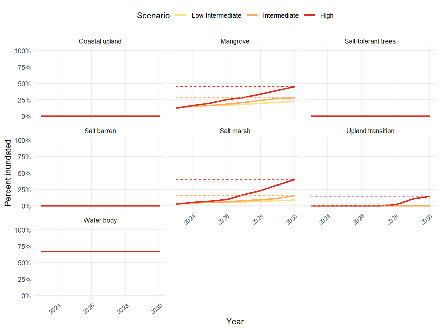
maxyr <- 2030
toplo2 <- zoneinund %>% 
  filter(yrs <= maxyr)
perinund <- toplo2 %>% 
  filter(yrs == maxyr) %>% 
  mutate(
    labs = paste0(round(100 * perinund, 0), '%')
  )
ggplot(toplo2, aes(x = yrs, y = perinund, color = scenario, group = scenario)) +
  geom_line(linewidth = 1) +
  geom_segment(data = perinund, aes(xend = yrs, y = perinund, yend = perinund, color = scenario), linetype = 'dashed', x = 2023) +
  facet_wrap(~Simplified_zone_name) +
  scale_color_manual(values = scencols) +
  scale_y_continuous(labels = scales::percent) +
  coord_cartesian(ylim = c(0, 1)) +
  theme_minimal() + 
  theme(
    panel.grid.minor = element_blank(),
    legend.position = 'top',
    axis.text.x = element_text(angle = 40, hjust = 1, size = 8)
  ) + 
  labs(
    x = 'Year',
    y = 'Percent inundated',
    color = 'Scenario'
  )

Percent of CCHA zones inundated from 2023 to 2030 for three scenarios. Horizontal dashed lines show the estimated percent at 2030. Assumes no accretion nor inland migration.

2050 - HMP goals

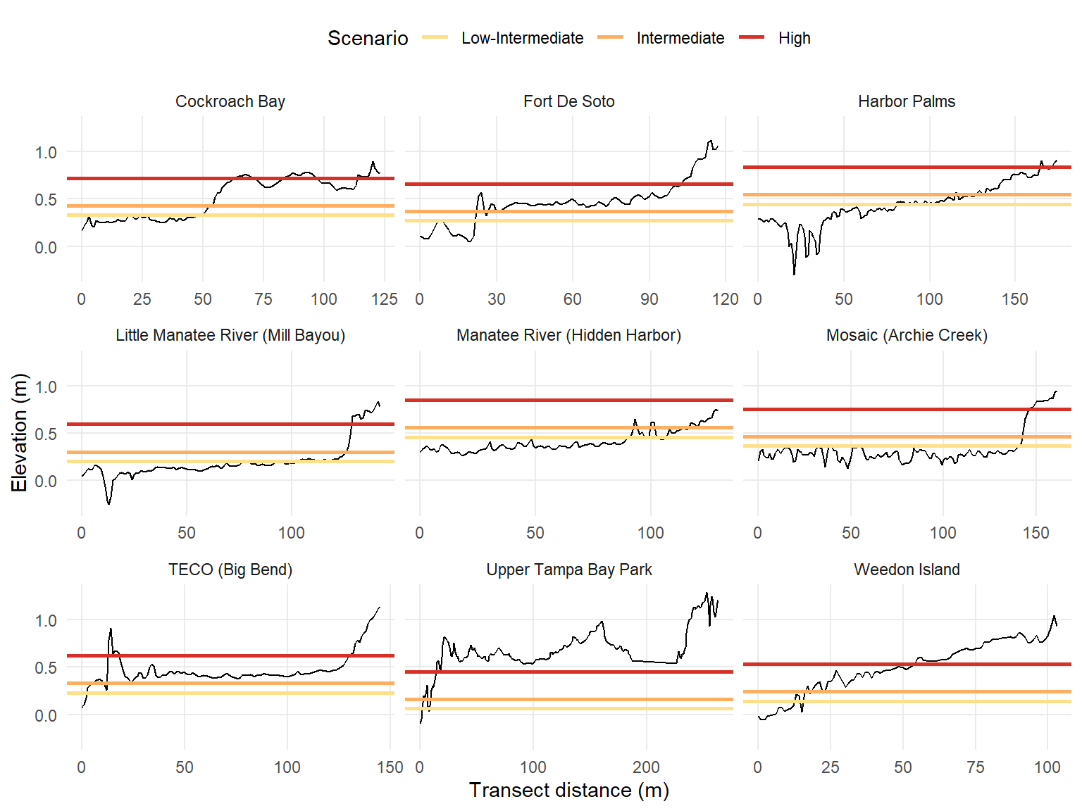
toplo1 <- jndat %>% 
  filter(yrs %in% c(2050))

ggplot(toplo1, aes(x = Meter, y = Elevation_NAVD88)) + 
  geom_line() +
  facet_wrap(~Site, scales = 'free_x') +
  geom_hline(aes(yintercept = MSL_m, color = scenario), linewidth = 1) +
  scale_color_manual(values = scencols) +
  theme_minimal() +
  theme(
    panel.grid.minor = element_blank(),
    legend.position = 'top'
  ) + 
  labs(
    x = 'Transect distance (m)',
    y = 'Elevation (m)',
    color = 'Scenario'
  )

Projected relative sea level rise in 2050 for three scenarios by CCHA transect. Assumes no accretion nor inland migration.

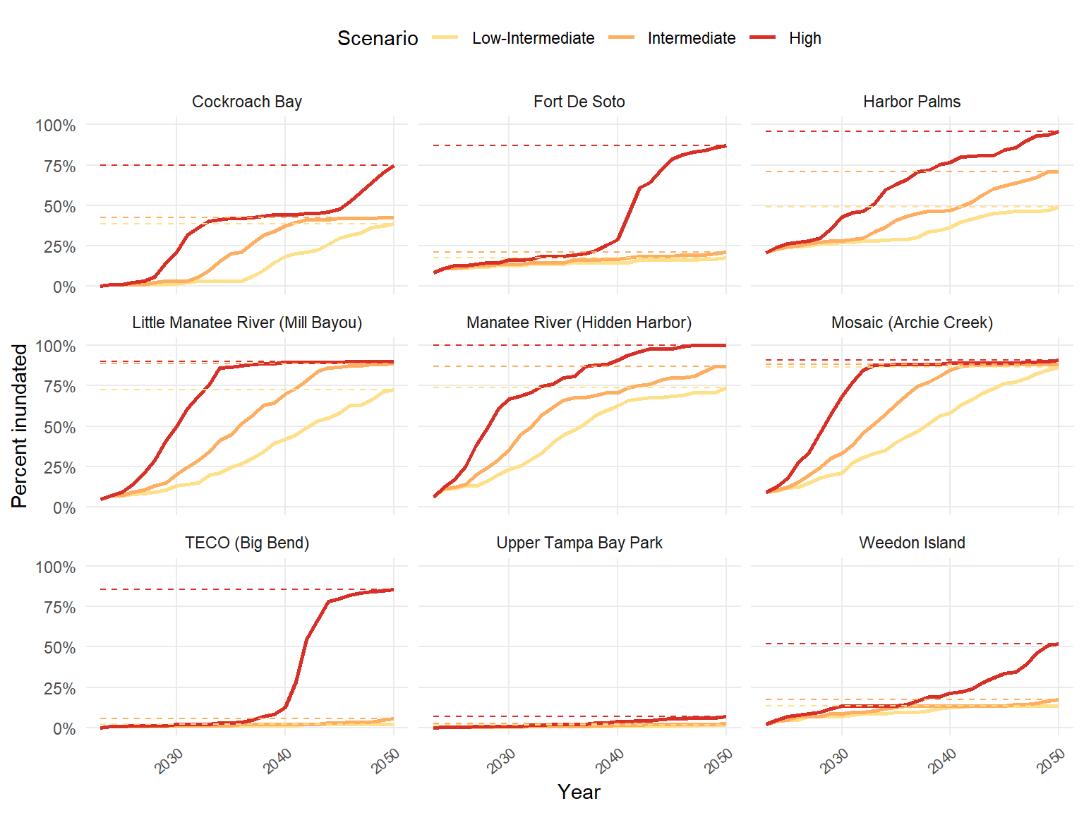
maxyr <- 2050
toplo2 <- inund %>% 
  filter(yrs <= maxyr)
perinund <- toplo2 %>% 
  filter(yrs == maxyr) %>% 
  mutate(
    labs = paste0(round(100 * perinund, 0), '%')
  )

ggplot(toplo2, aes(x = yrs, y = perinund, color = scenario, group = scenario)) +
  geom_line(linewidth = 1) +
  geom_segment(data = perinund, aes(xend = yrs, y = perinund, yend = perinund, color = scenario), linetype = 'dashed', x = 2023) +
  facet_wrap(~Site) +
  scale_color_manual(values = scencols) +
  scale_y_continuous(labels = scales::percent) +
  coord_cartesian(ylim = c(0, 1)) + 
  theme_minimal() + 
  theme(
    panel.grid.minor = element_blank(),
    legend.position = 'top',
    axis.text.x = element_text(angle = 40, hjust = 1, size = 8)
  ) + 
  labs(
    x = 'Year',
    y = 'Percent inundated',
    color = 'Scenario'
  )

Percent of CCHA transect inundated from 2023 to 2050 for three scenarios. Horizontal dashed lines show the estimated percent at 2050. Assumes no accretion nor inland migration.

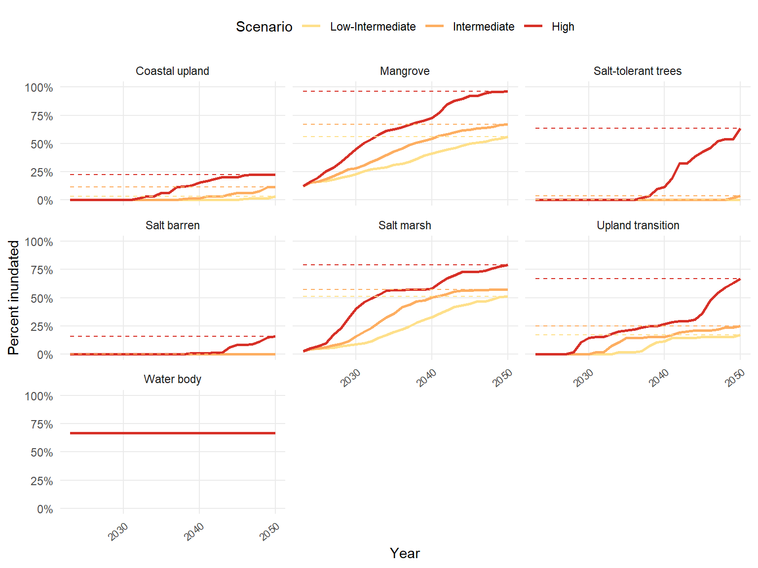
maxyr <- 2050
toplo2 <- zoneinund %>% 
  filter(yrs <= maxyr)
perinund <- toplo2 %>% 
  filter(yrs == maxyr) %>% 
  mutate(
    labs = paste0(round(100 * perinund, 0), '%')
  )
ggplot(toplo2, aes(x = yrs, y = perinund, color = scenario, group = scenario)) +
  geom_line(linewidth = 1) +
  geom_segment(data = perinund, aes(xend = yrs, y = perinund, yend = perinund, color = scenario), linetype = 'dashed', x = 2023) +
  facet_wrap(~Simplified_zone_name) +
  scale_color_manual(values = scencols) +
  scale_y_continuous(labels = scales::percent) +
  coord_cartesian(ylim = c(0, 1)) +
  theme_minimal() + 
  theme(
    panel.grid.minor = element_blank(),
    legend.position = 'top',
    axis.text.x = element_text(angle = 40, hjust = 1, size = 8)
  ) + 
  labs(
    x = 'Year',
    y = 'Percent inundated',
    color = 'Scenario'
  )

Percent of CCHA zones inundated from 2023 to 2050 for three scenarios. Horizontal dashed lines show the estimated percent at 2050. Assumes no accretion nor inland migration.

2100

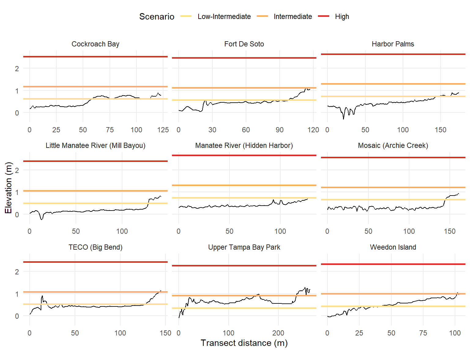
toplo1 <- jndat %>% 
  filter(yrs %in% c(2100))

ggplot(toplo1, aes(x = Meter, y = Elevation_NAVD88)) + 
  geom_line() +
  facet_wrap(~Site, scales = 'free_x') +
  geom_hline(aes(yintercept = MSL_m, color = scenario), linewidth = 1) +
  scale_color_manual(values = scencols) +
  theme_minimal() +
  theme(
    panel.grid.minor = element_blank(),
    legend.position = 'top'
  ) + 
  labs(
    x = 'Transect distance (m)',
    y = 'Elevation (m)',
    color = 'Scenario'
  )

Projected relative sea level rise in 2100 for three scenarios by CCHA transect. Assumes no accretion nor inland migration.

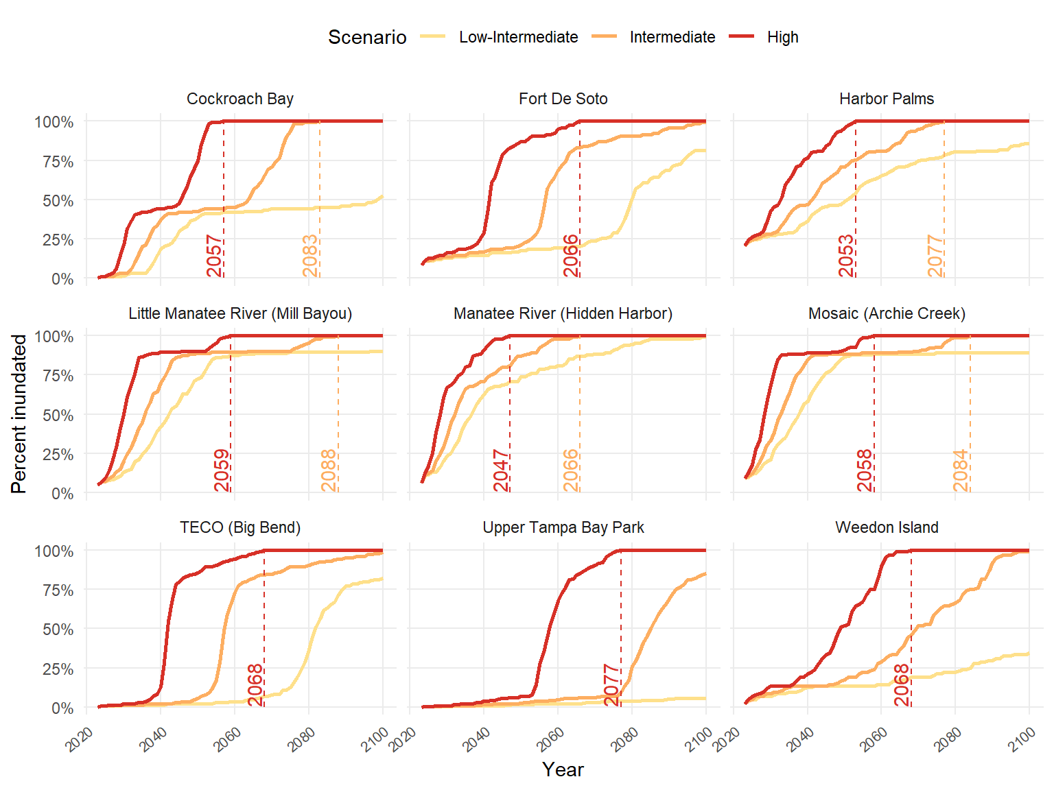
inundyr <- inund %>% 
  filter(perinund >= 1) %>% 
  filter(yrs == min(yrs), .by = c(Site, scenario))
ggplot(inund, aes(x = yrs, y = perinund, color = scenario, group = scenario)) +
  geom_line(linewidth = 1) +
  geom_segment(data = inundyr, aes(x = yrs, xend = yrs, y = 0, yend = 1, color = scenario), linetype = 'dashed') +
  geom_text(data = inundyr, aes(label = yrs, x = yrs), y = 0, hjust = 0, vjust = -0.2, angle = 90, show.legend = F) +
  facet_wrap(~Site) +
  scale_color_manual(values = scencols) +
  scale_y_continuous(labels = scales::percent) +
  theme_minimal() + 
  theme(
    panel.grid.minor = element_blank(),
    legend.position = 'top',
    axis.text.x = element_text(angle = 40, hjust = 1, size = 8)
  ) + 
  labs(
    x = 'Year',
    y = 'Percent inundated',
    color = 'Scenario'
  )

Percent of CCHA transect inundated from 2023 to 2100 for three scenarios. Estimated year of inundation for each scenario is shown on the bottom of each facet. Assumes no accretion nor inland migration.

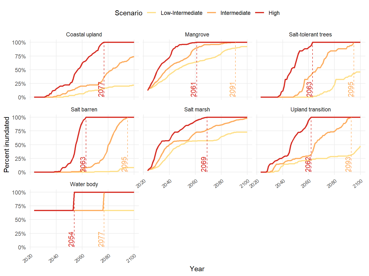
inundyr <- zoneinund %>% 
  filter(perinund >= 1) %>% 
  filter(yrs == min(yrs), .by = c(Simplified_zone_name, scenario))
ggplot(zoneinund, aes(x = yrs, y = perinund, color = scenario, group = scenario)) +
  geom_line(linewidth = 1) +
  geom_segment(data = inundyr, aes(x = yrs, xend = yrs, y = 0, yend = 1, color = scenario), linetype = 'dashed') +
  geom_text(data = inundyr, aes(label = yrs, x = yrs), y = 0, hjust = 0, vjust = -0.2, angle = 90, show.legend = F) +
  facet_wrap(~Simplified_zone_name) +
  scale_color_manual(values = scencols) +
  scale_y_continuous(labels = scales::percent) +
  theme_minimal() + 
  theme(
    panel.grid.minor = element_blank(),
    legend.position = 'top',
    axis.text.x = element_text(angle = 40, hjust = 1, size = 8)
  ) + 
  labs(
    x = 'Year',
    y = 'Percent inundated',
    color = 'Scenario'
  )

Percent of CCHA zones inundated from 2023 to 2100 for three scenarios. Estimated year of inundation for each scenario is shown on the bottom of each facet. Assumes no accretion nor inland migration.