Manuscript figures

library(tidyverse)
library(patchwork)
library(dplyr)
library(purrr)
library(tidyr)
library(ggplot2)
library(here)
library(ggalluvial)

load(file = here::here('data/tempdat.RData'))
vegdatelezcomp <- read.csv(here::here('data/raw/vegdatelezcomp.csv'))
vegdatele <- read.csv(here('data/raw/vegdatele.csv'))

rlefun <- function(x){
  runs <- rle(x)
  if(!any(runs$values)) return(0)
  max(runs$lengths[runs$values])
}

yrstr <- 1980

toplo <- tempdat |> 
  mutate(
    date = lubridate::ymd_hms(date), 
    yr = lubridate::year(date), 
    below = value < 0
  ) |> 
  filter(yr >= yrstr) |>
  summarize(
    temp = min(value), 
    nbelow = sum(below), 
    ncont = rlefun(below), 
    .by = yr
  )

toplo1 <- toplo
p1 <- ggplot(toplo1, aes(x = yr, y = temp)) +  
  geom_line() + 
  geom_point() +
  geom_hline(aes(color = "Mangrove threshold", yintercept = -4), linetype = "dashed") +
  scale_x_continuous(expand = c(0.1, 0.1)) + 
  scale_y_continuous(breaks = scales::pretty_breaks()) +
  scale_color_manual(values = "cyan3") +
  coord_cartesian(xlim = c(1978, 2026), expand = F) +
  theme_minimal() + 
  labs(
    x = NULL,
    color = NULL,
    y = 'Minimum air temp (°C)'
  )

toplo2 <- toplo |> 
  select(-temp) |> 
  pivot_longer(
    cols = -yr, 
    names_to = 'var', 
    values_to = 'value'
  ) |> 
  mutate(var = factor(var, levels = c('ncont', 'nbelow'), 
    labels = c('Longest cold spell', 'Total days')))

p2 <- ggplot(toplo2, aes(x = yr, y = value, fill = var)) + 
  geom_bar(stat = 'identity') + 
  scale_fill_manual(values = c('deepskyblue4', 'deepskyblue1')) +
  scale_y_continuous(breaks = scales::pretty_breaks()) +
  coord_cartesian(xlim = c(1978, 2026), expand = F) +
  theme_minimal() +
  labs(
    x = NULL,
    fill = NULL,
    y = 'Number of days\nbelow freezing'
  )

p <- p1 + p2 + 
  plot_layout(ncol = 1, height = c(2, 1), guides = 'collect') &
  theme(legend.position = 'bottom')

p

Annual minimum daily air temperature and freezing days in Tampa, Florida (1980 - 2024). Top panel shows annual minimum daily air temperature with dashed line indicating mangrove cold tolerance threshold (Cavanaugh et al. 2014). Bottom panel shows total number of days below freezing (light blue) and longest consecutive cold spell (dark blue) per year. Air temperature data from Tampa International Airport (NOAA NCEI station USW00012842)

# # accretion rates, based on RTK elevation diff per year  
# accrt <- vegdatele %>%
#   mutate(
#     yr = year(mdy(Date))
#   ) %>% 
#   summarise(
#     meanele = mean(Elevation_NAVD88, na.rm = T), 
#     .by = c(Site, yr)
#   ) %>% 
#   summarise(
#     elediff = diff(meanele), 
#     yrdiff = diff(yr), 
#     .by = Site
#   ) %>% 
#   mutate(
#     accrate = elediff / yrdiff
#   ) %>% 
#   select(Site, accrate)

ele <- vegdatelezcomp %>% 
  filter(Sample_set == 3) %>% 
  select(Site, Simplified_zone_name, Meter, Elevation_MTL) %>% 
  distinct() |> 
  mutate(
    zone_group = cumsum(Simplified_zone_name != lag(Simplified_zone_name, default = first(Simplified_zone_name))) + 1,
    .by = Site
  )

interpolate_transect <- function(df) {
  
  # Process each site separately
  df_interpolated <- df %>%
    group_by(Site) %>%
    do({
      site_data <- .
      
      # Create the new meter sequence at 0.25m intervals
      meter_seq <- seq(from = min(site_data$Meter), 
                      to = max(site_data$Meter), 
                      by = 0.1)
      
      # Create a new dataframe with the interpolated meter values
      new_df <- data.frame(
        Site = unique(site_data$Site),
        Meter = meter_seq
      )
      
      # Interpolate elevation using linear interpolation
      new_df$Elevation_MTL <- approx(x = site_data$Meter, 
                                     y = site_data$Elevation_MTL, 
                                     xout = meter_seq, 
                                     method = "linear")$y
      
      # For categorical variables, use "last observation carried forward"
      # This assumes zones are continuous until they change
      
      # First, create a mapping of meter to zone values
      zone_df <- site_data %>%
        select(Meter, Simplified_zone_name, zone_group)
      
      # Merge and fill forward the categorical values
      new_df <- new_df %>%
        left_join(zone_df, by = "Meter") %>%
        arrange(Meter) %>%
        fill(Simplified_zone_name, zone_group, .direction = "down")
      
      new_df
    }) %>%
    ungroup()
  
  return(df_interpolated)
}

toplo <- interpolate_transect(ele) 

toplo2 <- toplo |> 
  unite(zone_group, c('Site', 'zone_group'), sep = '_')

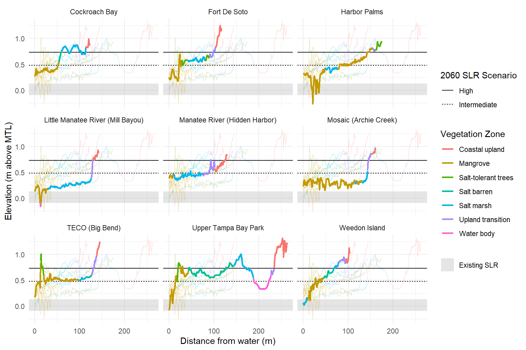
lns <- tibble(
  Scenario = c('High', 'Intermediate'),
  elev = c(0.73, 0.48)
)

rects <- tibble(
  Site = unique(toplo$Site),
  ymin = -0.095,
  ymax = 0.129
)

p <- ggplot(toplo, aes(x = Meter, y = Elevation_MTL, color = Simplified_zone_name, group = zone_group)) +
  geom_rect(data = rects, aes(ymin = ymin, ymax = ymax, fill = 'Existing SLR', xmin = -Inf, xmax = Inf), alpha = 0.4, inherit.aes = F) +
  geom_line(data = toplo2, aes(x = Meter, y = Elevation_MTL, group = 
    zone_group, color = Simplified_zone_name), alpha = 0.2) +
  geom_hline(data = lns, aes(yintercept = elev, linetype = Scenario), color = 'black') +
  geom_line(size = 1) + 
  scale_fill_manual(values = 'grey') +
  facet_wrap(~ Site) +
  theme_minimal() +
#   theme(
#     legend.position = "bottom"
#   ) +
  labs(
    x = "Distance from water (m)", 
    y = "Elevation (m above MTL)", 
    color = "Vegetation Zone", 
    fill = NULL, 
    linetype = '2060 SLR Scenario'
  )
p

Vegetation zones and elevations along site transects. Black lines indicate projected sea level rise by 2060 under high and intermediate scenarios (Sweet et al. 2022). Shaded gray area indicates existing sea level rise from historical tidal gauge data.

dat <- vegdatele |> 
  arrange(Site, Sample_set, Meter) |>
  group_nest(Site) |>
  mutate(
    data = map(data, function(x){

      filledzwide <- x |> 
        select(Sample_set, Meter, Simplified_zone_name) |> 
        distinct() |> 
        complete(Sample_set, Meter) |> 
        fill(Simplified_zone_name) |> 
        pivot_wider(names_from = Sample_set, values_from = Simplified_zone_name, values_fn = ~.x[1])

      out <- left_join(x, filledzwide, by = 'Meter')
      
      return(out)
      
    })
  ) |> 
  unnest(data) |> 
  select(site = Site, meter = Meter, `1`, `3`) |> 
  pivot_longer(cols = c(`1`, `3`), names_to = 'sample', values_to = 'zonefct') |> 
  unique() |> 
  arrange(site, sample, meter) |> 
  group_nest(site, sample) |> 
  mutate(
    data = map(data, function(x){
      
      rle_result <- rle(x$zonefct)
      letters_vector <- letters[1:length(rle_result$values)]
      result_vector <- rep(letters_vector, rle_result$lengths)
      
      x$lets <- result_vector
      
      return(x)
      
    })
  ) |> 
  unnest('data') |> 
  unite('lets', c('sample', 'lets'), sep = '_', remove = F) |> 
  mutate(zonefct = factor(zonefct)) |> 
  filter(!grepl('\\.5$', meter)) |> 
  mutate(
    sample = factor(sample, levels = c('1', '3'), labels = c('Baseline', '2023'))
  )

toplo <- dat

cols <- function(n) {
  hues = seq(15, 375, length = n + 1)
  hcl(h = hues, l = 65, c = 100)[1:n]
}
levs <- levels(toplo$zonefct)
colin <- cols(length(levs))
names(colin) <- levs

ggplot(toplo, aes(x = meter, y = sample, group = lets)) + 
  geom_line(aes(color = zonefct), stat = 'identity', lwd = 15, alpha = 0.7) + 
  scale_x_continuous(breaks = seq(0, max(toplo$meter), by = 20), expand = c(0, 0)) +
  guides(color = guide_legend(override.aes = list(lwd = 7))) +
  scale_colour_manual(values = colin, limits = force) +
  facet_wrap(~site, scales = 'free_x', ncol = 3) +
  theme_minimal() +
  theme(
    panel.grid.major.y = element_blank(), 
    legend.position = 'top', 
    panel.spacing.x = unit(1, 'lines'), 
    axis.text.x = element_text(size = 7)
  ) +
  labs(
    x = 'Meters', 
    color = 'Vegetation Zone',
    y = NULL
  )

Vegetation zone shifts across all transects from baseline surveys (2014 – 2016) to 2023.

toplo <- dat

cols <- function(n) {
  hues = seq(15, 375, length = n + 1)
  hcl(h = hues, l = 65, c = 100)[1:n]
}
levs <- levels(toplo$zonefct)
colin <- cols(length(levs))
names(colin) <- levs

ggplot(toplo,
            aes(x = sample, stratum = zonefct, alluvium = meter,
                y = 1, fill = zonefct, label = zonefct)) +
  geom_flow(stat = "alluvium", lode.guidance = "frontback") +
  geom_stratum() +
  scale_fill_manual(values = colin, limits = force) +
  facet_wrap(~site, scales = 'free_y') + 
  scale_x_discrete(expand = c(0.15, 0.15)) +
  theme_minimal() +
  theme(
    legend.position  = 'top', 
    panel.spacing.x = unit(1, 'lines'), 
    axis.text.y = element_blank(), 
    # axis.title.y = element_blank(),
    panel.grid = element_blank()
  ) +
  labs(
    x = NULL,
    fill = "Vegetation Zone",
    y = 'Relative change'
  )

Alluvial plots showing habitat shifts among vegetation zone types between baseline (2014 – 2016) and 2023 monitoring.

References

Cavanaugh, Kyle C, James R Kellner, Alexander J Forde, Daniel S Gruner, John D Parker, Wilfrid Rodriguez, and Ilka C Feller. 2014. “Poleward Expansion of Mangroves Is a Threshold Response to Decreased Frequency of Extreme Cold Events.” Proceedings of the National Academy of Sciences 111 (2): 723–27. https://doi.org/10.1073/pnas.1315800111.

Sweet, William V, Benjamin D Hamlington, Robert E Kopp, Christopher P Weaver, Patrick L Barnard, David Bekaert, William Brooks, et al. 2022. “Global and Regional Sea Level Rise Scenarios for the United States: Updated Mean Projections and Extreme Weather Level Probabilities Along US Coastlines.” NOS 01. Silver Spring, MD: National Oceanic; Atmospheric Administration, National Ocean Service.