Zone predictions for phase 2 CCHA sampling

Code

library(tidyverse)
library(randomForest)
library(janitor)
library(caret)
library(zoo)
library(here)

load(file = here('data/vegdat.RData'))

# colors
cols <- function(n) {
  hues = seq(15, 375, length = n + 1)
  hcl(h = hues, l = 65, c = 100)[1:n]
}
levs <- vegdat %>% 
  select(zone_name_simp) %>% 
  distinct() %>% 
  arrange(zone_name_simp) %>% 
  na.omit() %>% 
  pull()
colin <- cols(length(levs))
names(colin) <- levs

# smoothing function for prediction post-processing
smooth_fun <- function(prds, win = 3, align = 'left', fillna = F){
  
  levs <- levels(prds)
  prds <- as.character(prds)
  out <- rollapply(
    prds, 
    width = win, FUN = function(x){
      names(sort(table(x), decreasing = TRUE)[1])
    }, 
    align = align, fill = NA)
  
  if(fillna)
    out <- ifelse(is.na(out), prds, out)
  
  out <- factor(out, levels = levs)
  
  return(out)
  
}

# species in all three samples
shrspp <- vegdat %>% 
  select(sample, species) %>% 
  distinct() %>% 
  mutate(
    present = 1
  ) %>% 
  pivot_wider(names_from = sample, values_from = present, values_fill = 0) %>% 
  mutate(
    allpresent = ifelse(`1` + `2` + `3` == 3, 1, 0)
  ) %>% 
  filter(allpresent == 1) %>% 
  pull(species) %>% 
  sort()

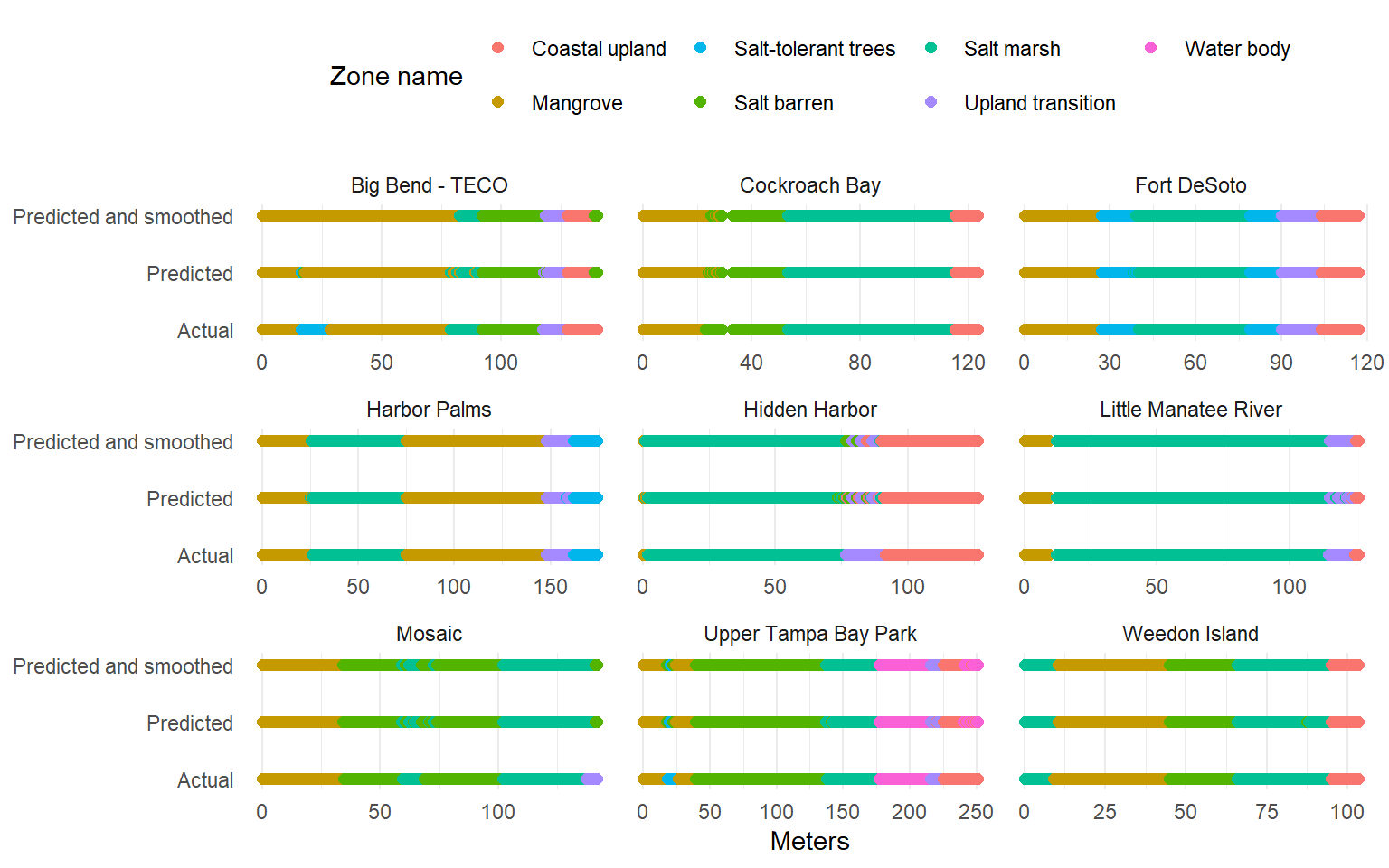
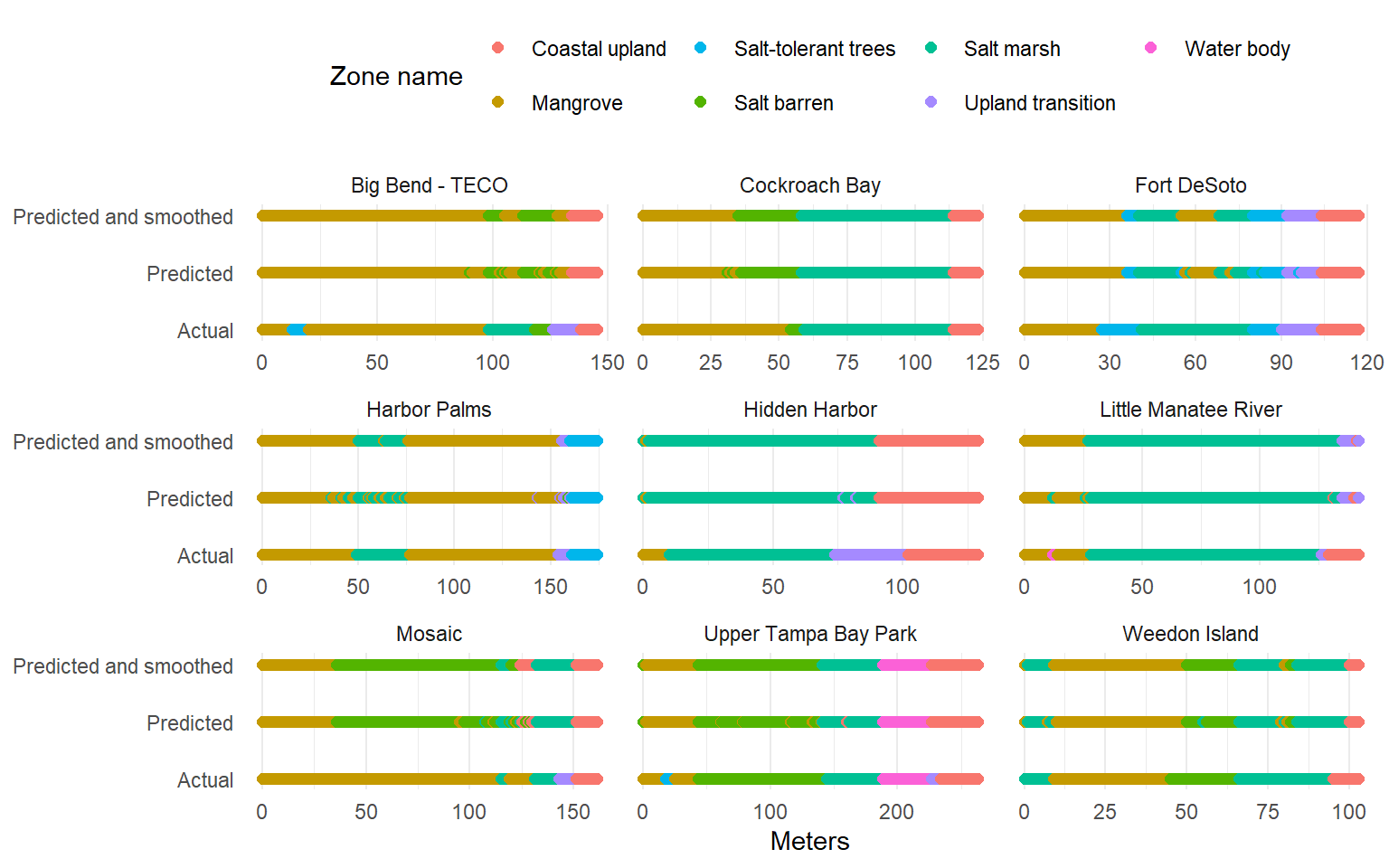
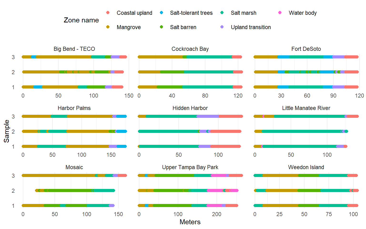
This analysis is a proof of concept for predicting vegetation zones in phase 2 sampling, where complete vegetation plots were sampled but no zone or elevation information was recorded. The predictions use a random forest model trained on the phase 1 data and tested on phase 3 data. The model used species basal percent cover, meter mark, and site as predictors. Only species shared across all three phases were included. The model predictions compared to actual zones for phase 1 (training) and phase 3 (validation) are shown for comparison, including model confusion matrices and accuracy statistics. Model predictions using smoothed results are also evaluated, where meter marks are assigned the majority zone within a rolling window of width 5.

Phase 1 training data

Code

# prep for rf, use first phase as training
trndat <- vegdat %>% 
  filter(species %in% shrspp) %>% 
  filter(sample == 1) %>% 
  select(
    site, zone_name_simp, meter, species, pcent_basal_cover
  ) %>% 
  summarise(
    pcent_basal_cover = mean(pcent_basal_cover, na.rm = T),
    .by = c(site, zone_name_simp, meter, species)
  ) %>% 
  filter(!is.na(pcent_basal_cover)) %>% 
  pivot_wider(names_from = species, values_from = pcent_basal_cover, values_fill = 0) %>% 
  clean_names() %>% 
  mutate_if(is.character, as.factor)

# rf mod
rfmod <- randomForest(zone_name_simp ~ ., data = trndat, importance = TRUE, ntree = 500, keep.inbag = T)

# data for checking results
trndatchk <- trndat %>% 
  mutate(
    zone_name_simpprd = predict(rfmod, .)
  ) %>% 
  select(
    site, 
    meter,
    zone_name_simp,
    zone_name_simpprd
  ) %>% 
  mutate(
    zone_name_simpprdsmth = smooth_fun(zone_name_simpprd, align = 'center', win = 5, fillna = T),
    .by = site
  )

Code

# visualize training results
toplo <- trndatchk %>% 
  pivot_longer(
    cols = -c(site, meter),
    names_to = 'typ',
    values_to = 'zone_name_simp'
  ) %>% 
  filter(!is.na(zone_name_simp)) %>% 
  mutate(
    typ = case_when(
      grepl('prd$', typ) ~ 'Predicted', 
      grepl('prdsmth$', typ) ~ 'Predicted and smoothed', 
      T ~ 'Actual'
    )
  )

ggplot(toplo, aes(x = meter, y = typ, color = zone_name_simp)) +
  geom_point(size = 2) +
  facet_wrap(~site, scales = 'free_x') +
  scale_color_manual(values = colin) +
  scale_y_discrete(expand = c(0.1, 0)) + 
  theme_minimal() +
  theme(
    legend.position = 'top',
    panel.grid.major.y = element_blank()
  ) +
  labs(
    x = 'Meters', 
    y = NULL, 
    color = 'Zone name'
  )

Model predictions for training data on phase 1 zones compared to actual.

Confusion matrix and accuracy statistic for model predictions compared to actual zones (reference).

Code

tmp1 <- confusionMatrix(trndatchk$zone_name_simpprd, trndatchk$zone_name_simp)
tmp1$table

                     Reference
Prediction            Coastal upland Mangrove Salt-tolerant trees Salt barren
  Coastal upland                 195        0                   0           0
  Mangrove                         0      646                  26           7
  Salt-tolerant trees              0        0                  76           0
  Salt barren                      3        2                  10         445
  Salt marsh                       0        5                   2           6
  Upland transition                1        0                   0           0
  Water body                      17        0                   0           0
                     Reference
Prediction            Salt marsh Upland transition Water body
  Coastal upland               0                 9          0
  Mangrove                     7                 0          0
  Salt-tolerant trees          0                 1          0
  Salt barren                 12                10          0
  Salt marsh                 904                15          0
  Upland transition            0               119          0
  Water body                   0                 0         78

Code

tmp1$overall['Accuracy']

 Accuracy 
0.9487673

Confusion matrix and accuracy statistic for smoothed model predictions compared to actual zones (reference).

Code

tmp2 <- confusionMatrix(trndatchk$zone_name_simpprdsmth, trndatchk$zone_name_simp)
tmp2$table

                     Reference
Prediction            Coastal upland Mangrove Salt-tolerant trees Salt barren
  Coastal upland                 191        0                   0           0
  Mangrove                         0      645                  29           7
  Salt-tolerant trees              0        0                  75           0
  Salt barren                      3        2                   8         446
  Salt marsh                       0        6                   2           5
  Upland transition                1        0                   0           0
  Water body                      21        0                   0           0
                     Reference
Prediction            Salt marsh Upland transition Water body
  Coastal upland               0                 7          0
  Mangrove                     7                 0          0
  Salt-tolerant trees          0                 0          0
  Salt barren                  5                12          0
  Salt marsh                 911                10          0
  Upland transition            0               125          0
  Water body                   0                 0         78

Code

tmp2$overall['Accuracy']

Accuracy 
0.951849

Phase 3 testing data

Code

# test dataset on phase 3
tstdat <- vegdat %>% 
  filter(sample == 3) %>% 
  select(
    site, zone_name_simp, meter, species, pcent_basal_cover
  ) %>% 
  summarise(
    pcent_basal_cover = mean(pcent_basal_cover, na.rm = T),
    .by = c(site, zone_name_simp, meter, species)
  ) %>% 
  pivot_wider(names_from = species, values_from = pcent_basal_cover, values_fill = 0) %>% 
  clean_names() %>% 
  mutate_if(is.character, as.factor)

tstdatchk <- tstdat %>% 
  mutate(
    zone_name_simpprd = predict(rfmod, .)
  ) %>% 
  select(
    site, 
    meter,
    zone_name_simp,
    zone_name_simpprd
  ) %>% 
  mutate(
    zone_name_simpprdsmth = smooth_fun(zone_name_simpprd, align = 'center', win = 5, fillna = T),
    .by = site
  )

Code

# visualize testing results
toplo <- tstdatchk %>% 
  pivot_longer(
    cols = -c(site, meter),
    names_to = 'typ',
    values_to = 'zone_name_simp'
  ) %>% 
  filter(!is.na(zone_name_simp)) %>% 
  mutate(
    typ = case_when(
      grepl('prd$', typ) ~ 'Predicted', 
      grepl('prdsmth$', typ) ~ 'Predicted and smoothed', 
      T ~ 'Actual'
    )
  )

ggplot(toplo, aes(x = meter, y = typ, color = zone_name_simp)) +
  geom_point(size = 2) +
  facet_wrap(~site, scales = 'free_x') +
  scale_color_manual(values = colin) +
  scale_y_discrete(expand = c(0.1, 0)) + 
  theme_minimal() +
  theme(
    legend.position = 'top',
    panel.grid.major.y = element_blank()
  ) +
  labs(
    x = 'Meters', 
    y = NULL, 
    color = 'Zone name'
  )

Model predictions for testing data on phase 3 zones compared to actual.

Confusion matrix and accuracy statistic for model predictions compared to actual zones (reference).

Code

tmp1 <- confusionMatrix(tstdatchk$zone_name_simpprd, tstdatchk$zone_name_simp)
tmp1$table

                     Reference
Prediction            Coastal upland Mangrove Salt-tolerant trees Salt barren
  Coastal upland                 108        4                   0           0
  Mangrove                         0      407                  23          13
  Salt-tolerant trees              0        0                  27           0
  Salt barren                      0      103                   0         116
  Salt marsh                      10       18                   2           5
  Upland transition                6        1                   0           0
  Water body                       0        0                   0           0
                     Reference
Prediction            Salt marsh Upland transition Water body
  Coastal upland               3                22          0
  Mangrove                    33                 8          0
  Salt-tolerant trees          1                 3          0
  Salt barren                 14                 3          0
  Salt marsh                 352                26          2
  Upland transition            0                17          0
  Water body                   0                 0         39

Code

tmp1$overall['Accuracy']

 Accuracy 
0.7803807

Confusion matrix and accuracy statistic for smoothed model predictions compared to actual zones (reference).

Code

tmp2 <- confusionMatrix(tstdatchk$zone_name_simpprdsmth, tstdatchk$zone_name_simp)
tmp2$table

                     Reference
Prediction            Coastal upland Mangrove Salt-tolerant trees Salt barren
  Coastal upland                 106        7                   0           0
  Mangrove                         0      411                  23           5
  Salt-tolerant trees              0        0                  28           0
  Salt barren                      0      104                   0         125
  Salt marsh                      11       11                   1           4
  Upland transition                7        0                   0           0
  Water body                       0        0                   0           0
                     Reference
Prediction            Salt marsh Upland transition Water body
  Coastal upland               1                22          0
  Mangrove                    27                 8          2
  Salt-tolerant trees          0                 3          0
  Salt barren                 14                 2          0
  Salt marsh                 361                28          0
  Upland transition            0                16          0
  Water body                   0                 0         39

Code

tmp2$overall['Accuracy']

Accuracy 
0.795022

Phase 2 predictions

Code

# predict sample 2
toprd <- vegdat %>% 
  filter(sample == 2) %>% 
  select(
    site, zone_name_simp, meter, species, pcent_basal_cover
  ) %>% 
  summarise(
    pcent_basal_cover = mean(pcent_basal_cover, na.rm = T),
    .by = c(site, zone_name_simp, meter, species)
  ) %>% 
  pivot_wider(names_from = species, values_from = pcent_basal_cover, values_fill = 0) %>% 
  clean_names() %>% 
  mutate_if(is.character, as.factor)

tomrg <- toprd %>% 
  mutate(
    sample = 2,
    zone_name_simp2 = predict(rfmod, newdata = .)
  ) %>% 
  mutate(
    zone_name_simp2 = smooth_fun(zone_name_simp2, align = 'center', win = 5, fillna = T),
    .by = site
  ) %>%
  select(site, sample, meter, zone_name_simp2) %>% 
  mutate(
    site = as.character(site),
    zone_name_simp2 = as.character(zone_name_simp2)
  ) 

vegdat2 <- vegdat %>% 
  group_nest(site, sample, zone_name_simp, meter) %>% 
  left_join(tomrg, by = c('site', 'sample', 'meter')) %>% 
  mutate(
    zone_name_simp = case_when(
      is.na(zone_name_simp) ~ zone_name_simp2, 
      T ~ zone_name_simp
    )
  ) %>% 
  select(-zone_name_simp2) %>%
  unnest('data') %>% 
  arrange(sample, site, meter, species)

Code

toplo <- vegdat2 %>% 
  select(site, sample, zone_name_simp, meter) %>%
  distinct() %>% 
  mutate(
    sample = factor(sample)
  )

ggplot(toplo, aes(x = meter, y = sample, color = zone_name_simp)) +
  geom_point(size = 2) +
  facet_wrap(~site, scales = 'free_x') +
  scale_color_manual(values = colin) +
  scale_y_discrete(expand = c(0.1, 0)) + 
  theme_minimal() +
  theme(
    legend.position = 'top',
    panel.grid.major.y = element_blank()
  ) +
  labs(
    x = 'Meters', 
    y = 'Sample', 
    color = 'Zone name'
  )

Site zones for all phases. Phases 1 and 3 are actual and phase 2 is predicted and smoothed.