chla ~ factor(bay_segment):factor(mo) + tn_load:factor(bay_segment)Exploring the Assimilative Capacity of Old Tampa Bay
Premise
Model 1 (Original), All Bay Segments
The cumulative lag model from Janicki and Wade 1996 is specified as:
\[ \text{chla}_{t, s} = \alpha_{t, s} + \beta_s \left( \Sigma_{i = I_0}^{I_n} L_{t - i, s} \right) \]
where \(\text{chla}_{t, s}\) is the chlorophyll-a concentration at month \(t\) and bay segment \(s\), \(\alpha_{t, s}\) is the intercept term that varies by \(t\) and \(s\), \(\beta_s\) is the coefficient for the cumulative load term that varies by \(s\), and \(L_{t - 1, s}\) is the cumulative nitrogen nitrogen load evaluated at different lags from \(I_0\) as the present month in the time series to \(I_n\) months for each \(s\).
Models are created with the following linear model structure in R, where the tn_load variable is the cumulative lag load for different \(n\) lags.
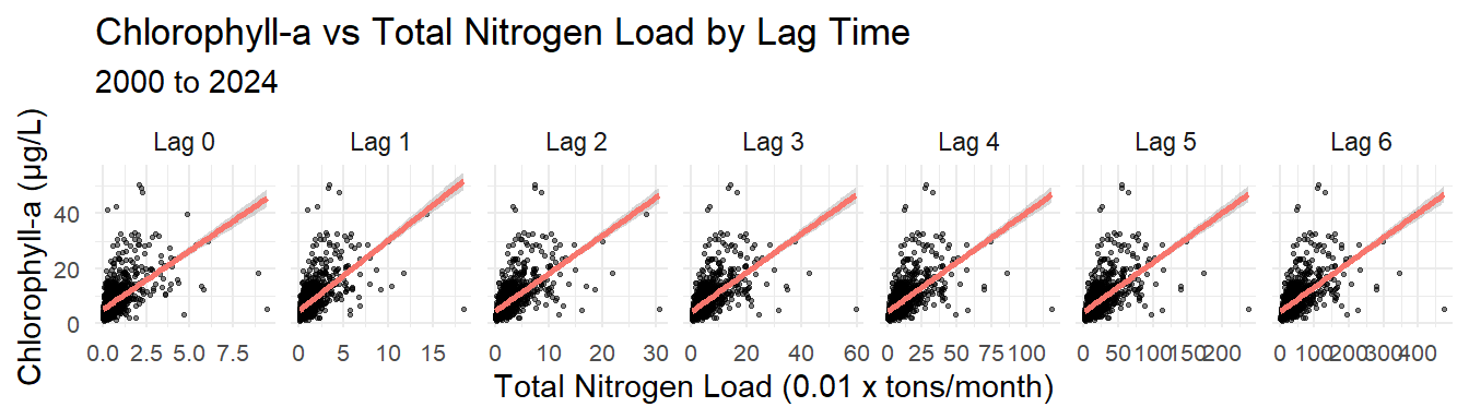
Model 1: OTB Only
The model is the same as above except the bay segment term is removed since only OTB is evaluated.
The cumulative lag model form is specified as:
\[ \text{chla}_{t} = \alpha_{t} + \beta \left( \Sigma_{i = I_0}^{I_n} L_{t - i} \right) \]
where \(\text{chla}_{t}\) is the chlorophyll-a concentration at month \(t\), \(\alpha_{t}\) is the intercept term that varies by \(t\), \(\beta\) is the coefficient for the cumulative load term, and \(L_{t - i}\) is the cumulative nitrogen load evaluated at different lags from \(I_0\) for the present month to \(I_n\) months.
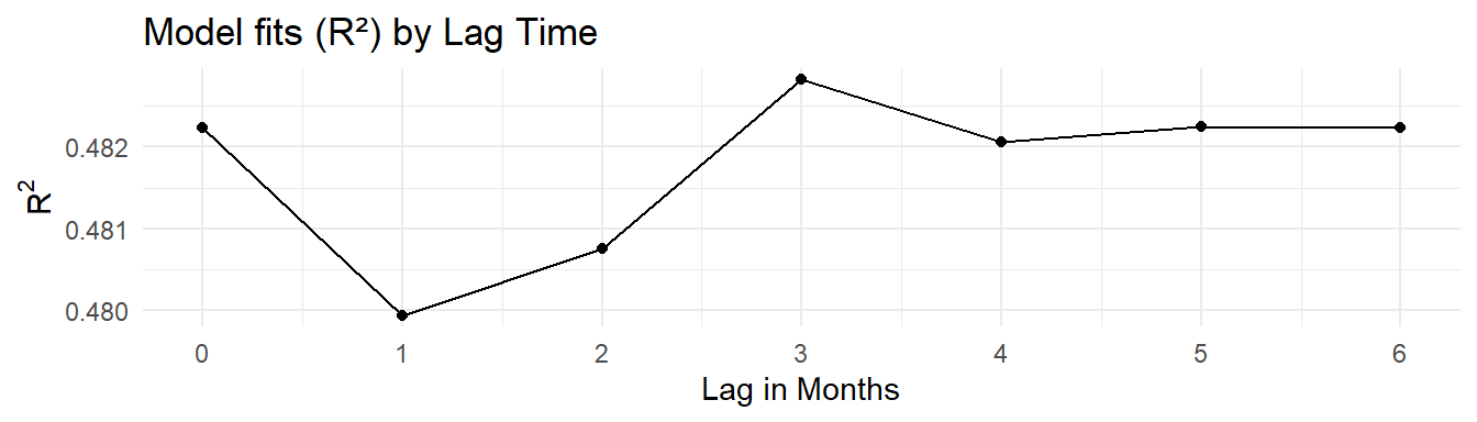
Models are run with the following linear model structure in R, where the tn_load variable is the cumulative lag load for different \(n\) lags.
chla ~ factor(mo) + tn_load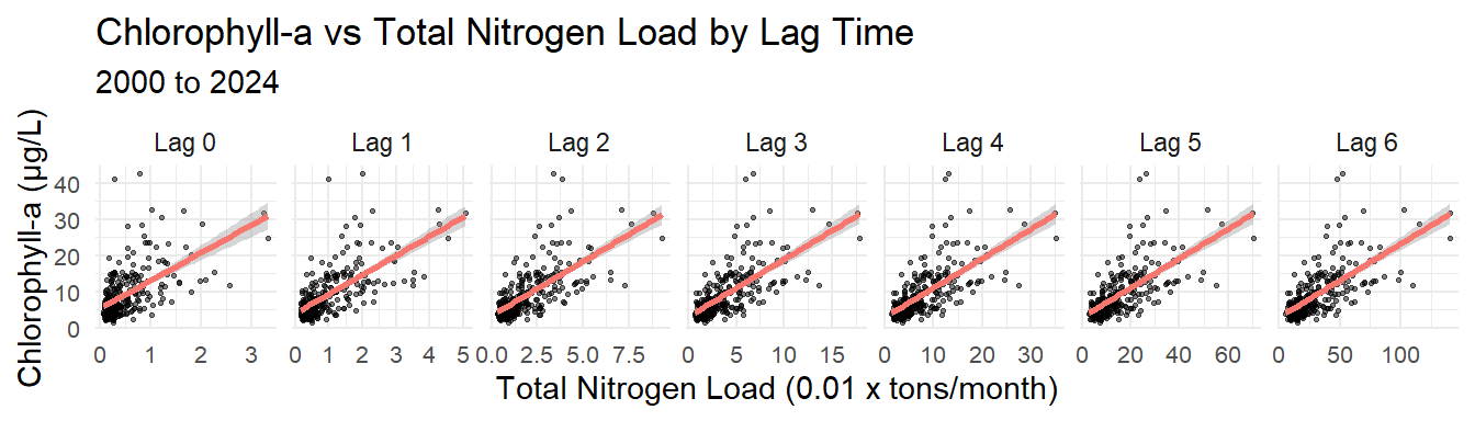
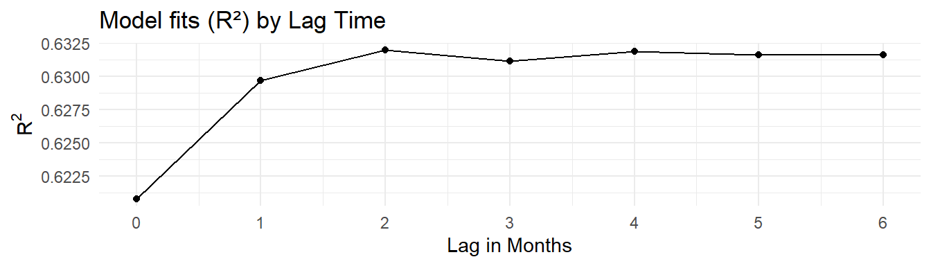
Model 1: Assimilative Capacity Analysis
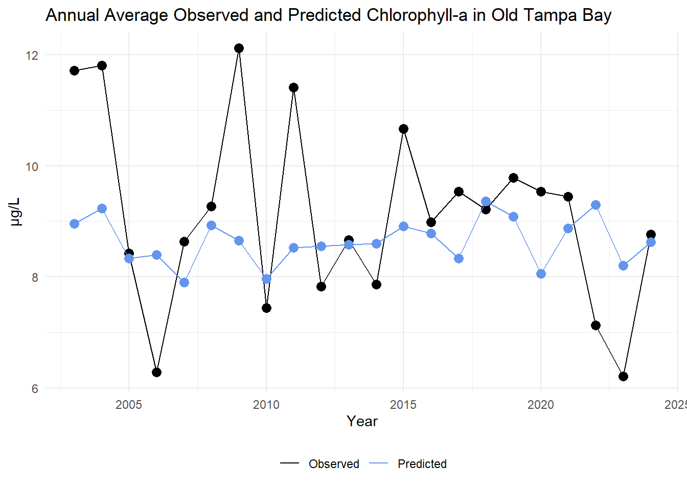
The cumulative lag model with a 3-month lag was chosen for the assimilative capacity analysis based on the results above and previous work by Janicki and Wade 1996.
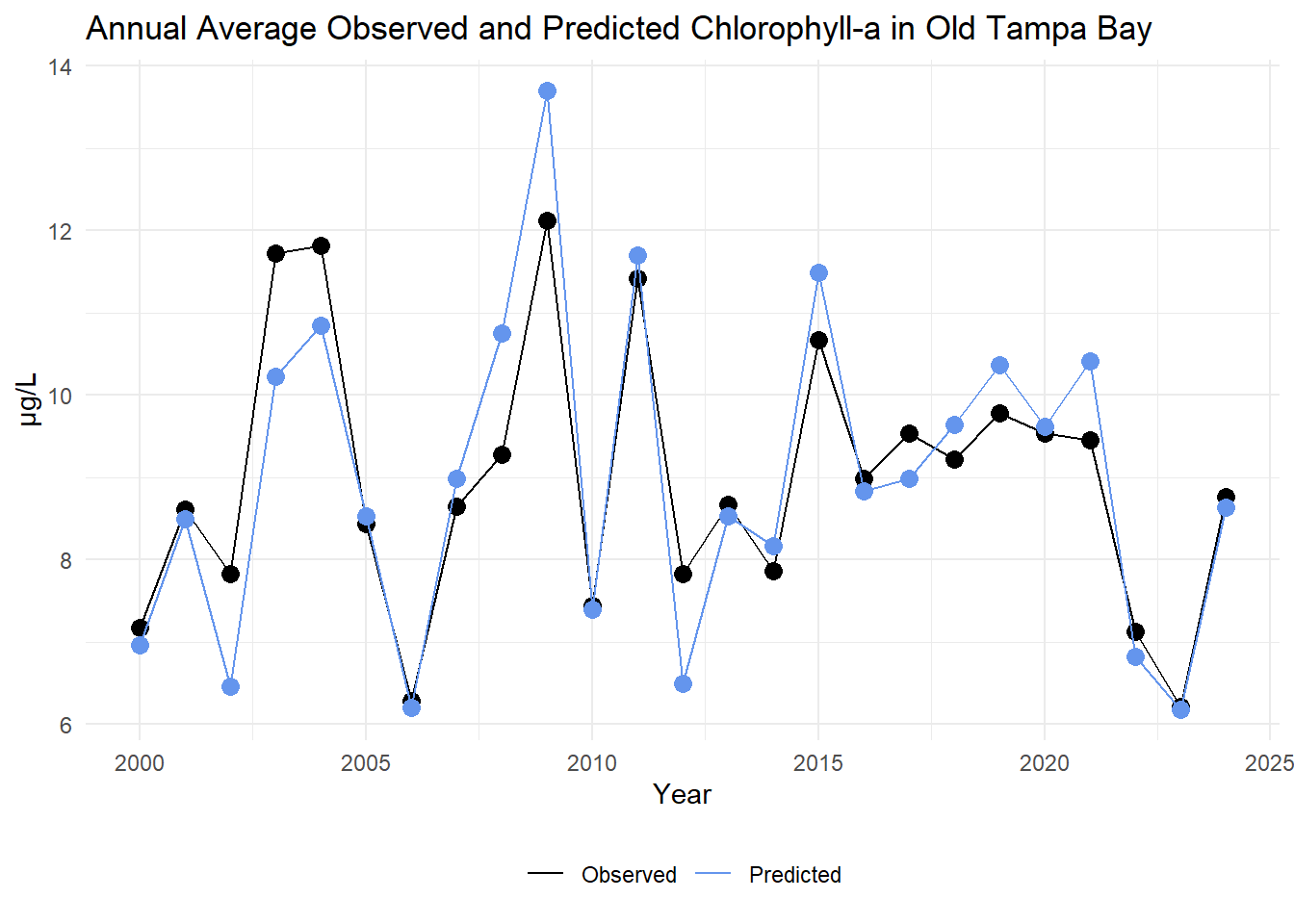
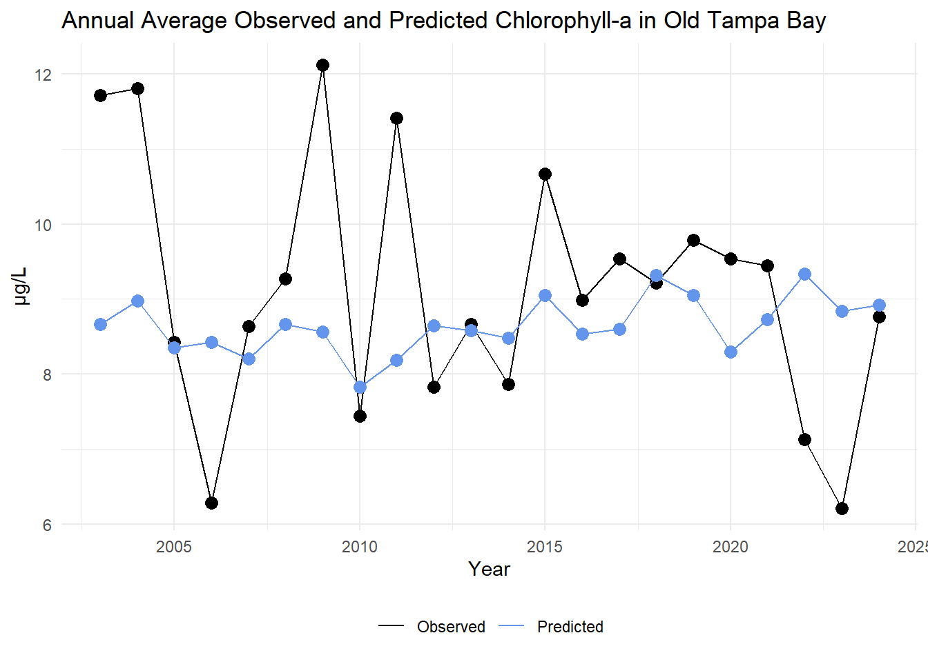
The annual average observed and predicted chlorophyll-a concentrations are compared for Old Tampa Bay below.
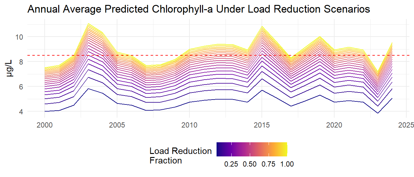
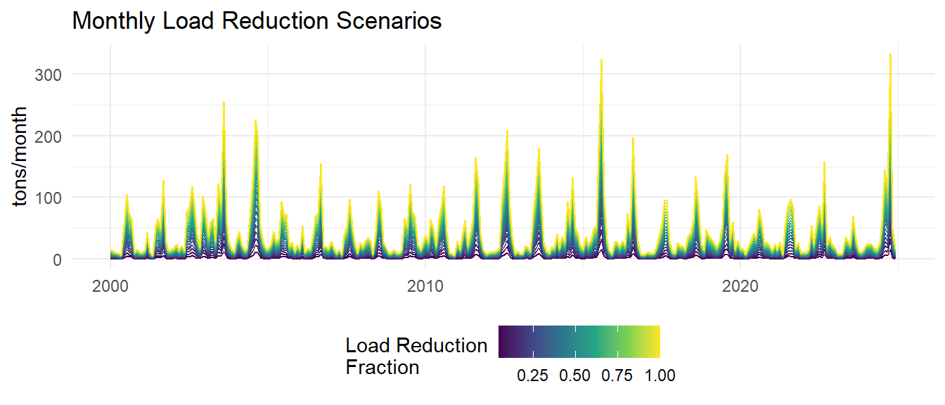
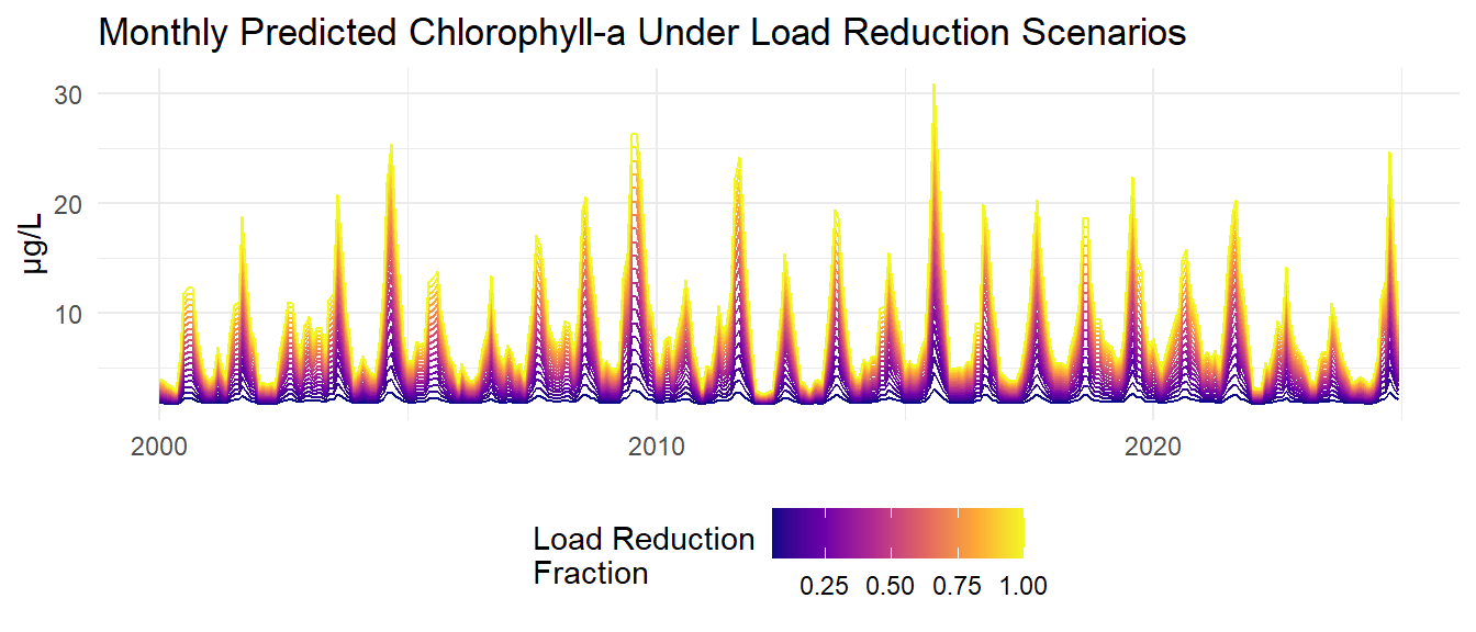
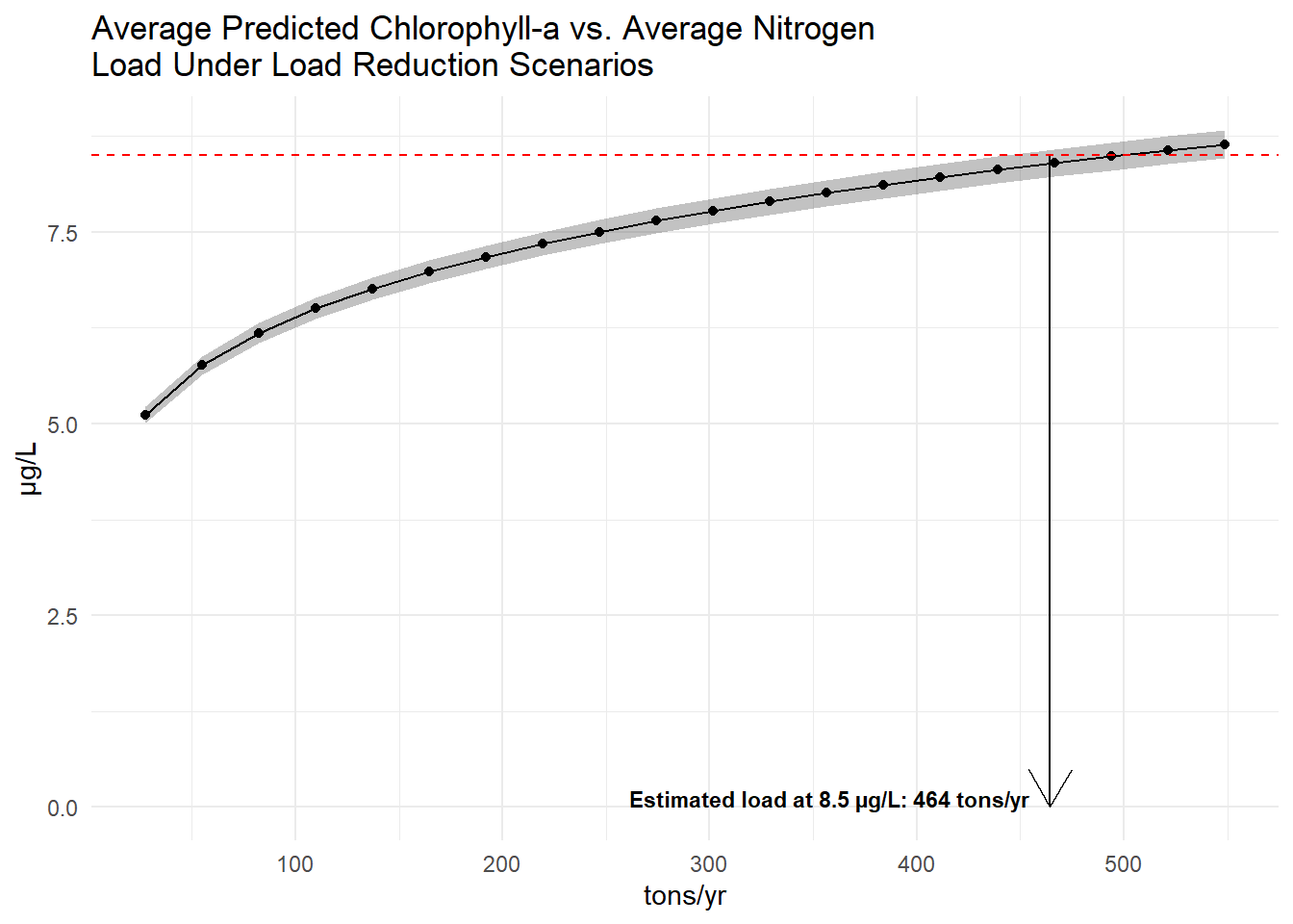
The assimilative capacity analysis involves simulating sequential nitrogen load reduction scenarios and predicting the resulting chlorophyll-a concentrations using the developed models. Monthly loads are reduced by fractions ranging from 5% to 100% in 5% increments. The models are then used to predict chlorophyll-a concentrations under each load reduction scenario.
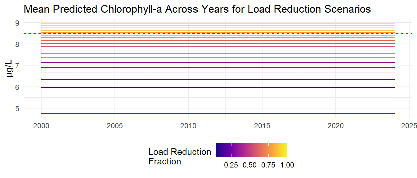
Monthly total nitrogen loads are then summed for the annual nitrogen loads and model predictions are aggregated to the annual average predicted chlorophyll-a concentrations for each load reduction scenario.

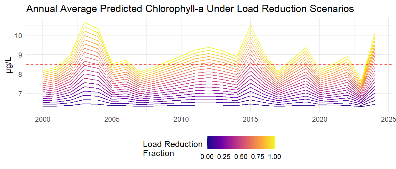
Annual load estimates and chlorophyll-a predictions for each load reduction scenario are then averaged across the years.
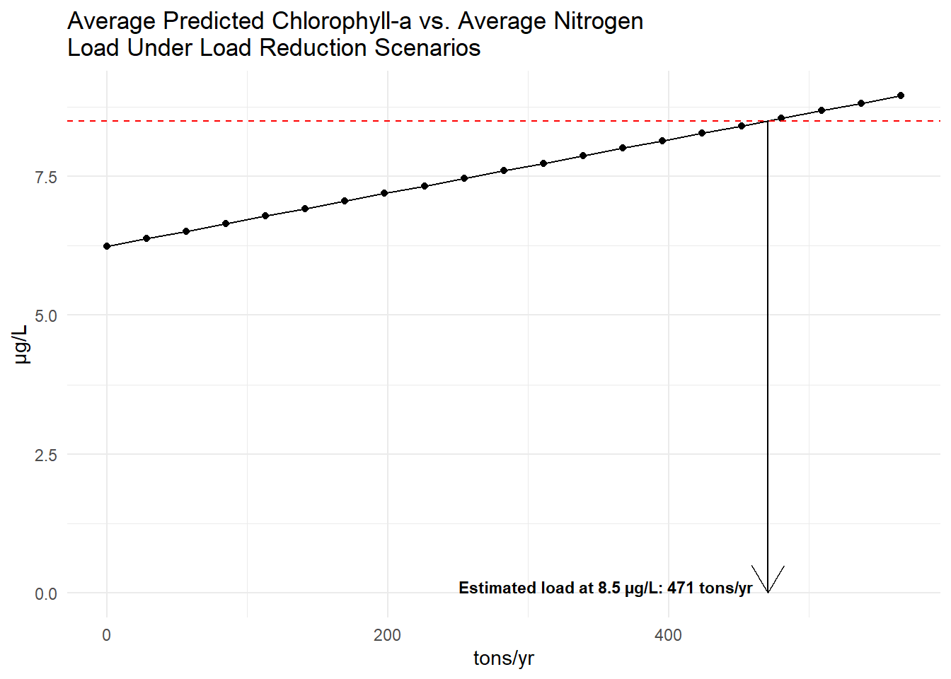

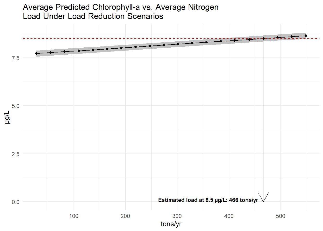
Plotting these averages against each other can demonstrate an expected response of chlorophyll to load changes for the model. The plot below shows each point as the average predicted chlorophyll-a versus the average total nitrogen load for each load reduction scenario. The dashed red line indicates the target chlorophyll-a concentration of 8.5 µg/L. The arrow indicates the estimated nitrogen load needed to achieve the target chlorophyll-a concentration based on linear interpolation of the average response curves. The estimated load needed to achieve 8.5 µg/L chlorophyll-a is 466 tons/year.
Model 2: Log-Model with Additional Predictors
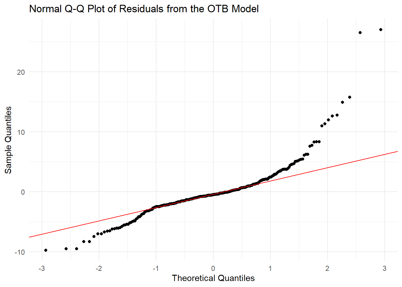
The above models used to predict the assimilative capacity of Old Tampa Bay, particularly for the period after 2010, likely provide an overestimate of how much loading the bay segment can assimilate. This is evident by evaluating the residual patterns - the model does not capture extreme values. Results could be improved by modeling an inherently log-normal response variable and including additional predictors to provide a more accurate estimate of how nitrogen load influences chlorophyll-a.
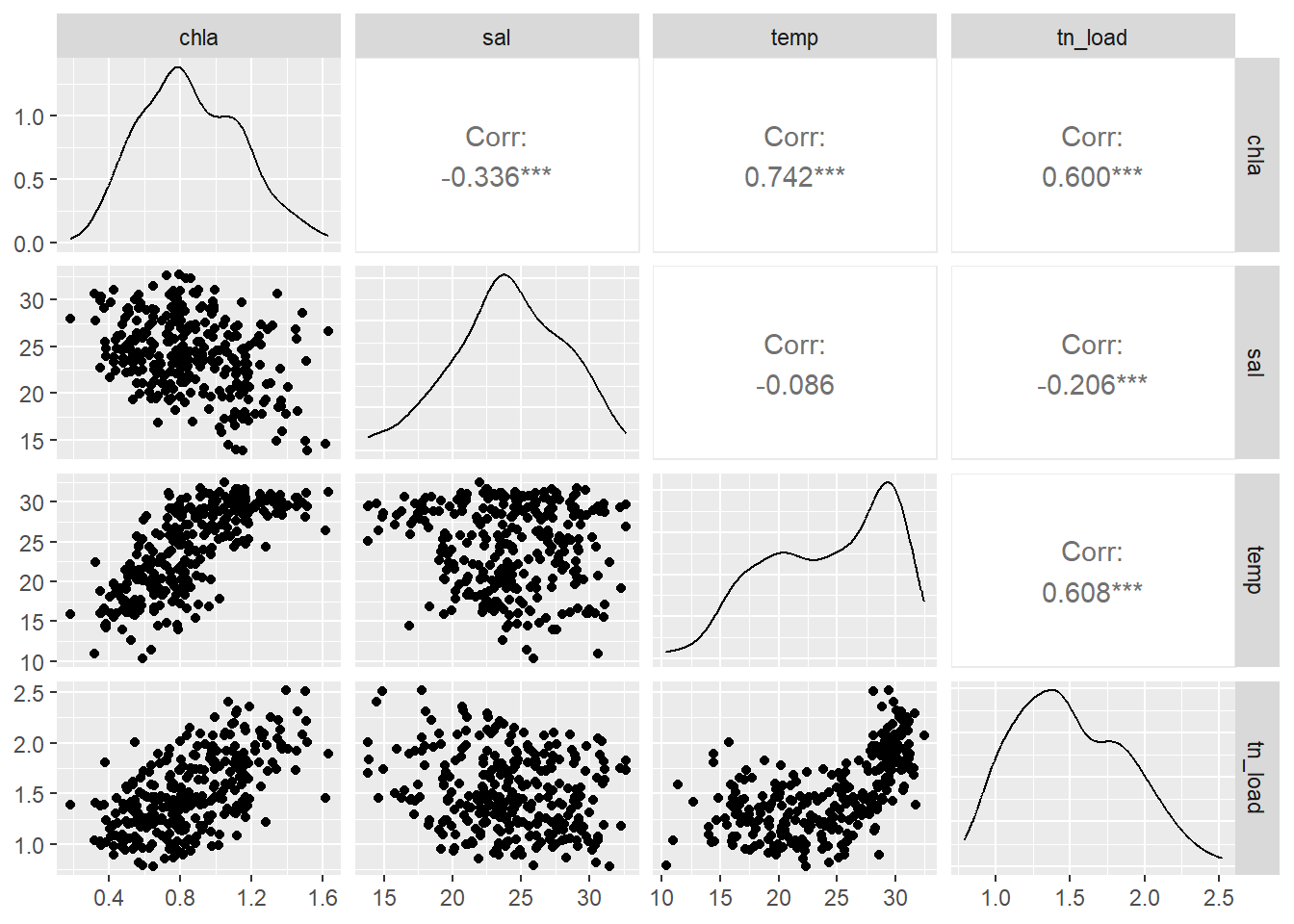
To address this issue, an additional model was developed using log-transformed chlorophyll-a as the response variable, log-transformed loading valuse, and additional predictors, including salinity and temperature.

Collinearity among the new predictors was assessed using variance inflation factors (VIFs), where chlorophyll and load are log-transformed. The values are sufficiently low to include all predictors in the model.
     sal     temp  tn_load
1.046733 1.589310 1.647133
The above analyses were repeated with the following changes to the model structure:
\[ log_{10}\text{chla}_{t} = \alpha_{t} + \beta_1 log_{10}\left( \Sigma_{i = I_0}^{I_n} L_{t - i} \right) + \beta_2 \text{sal}_{t} + \beta_3 \text{temp}_{t} \]
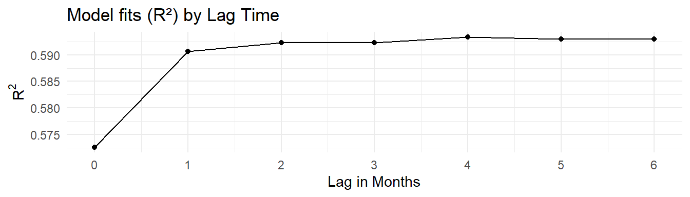
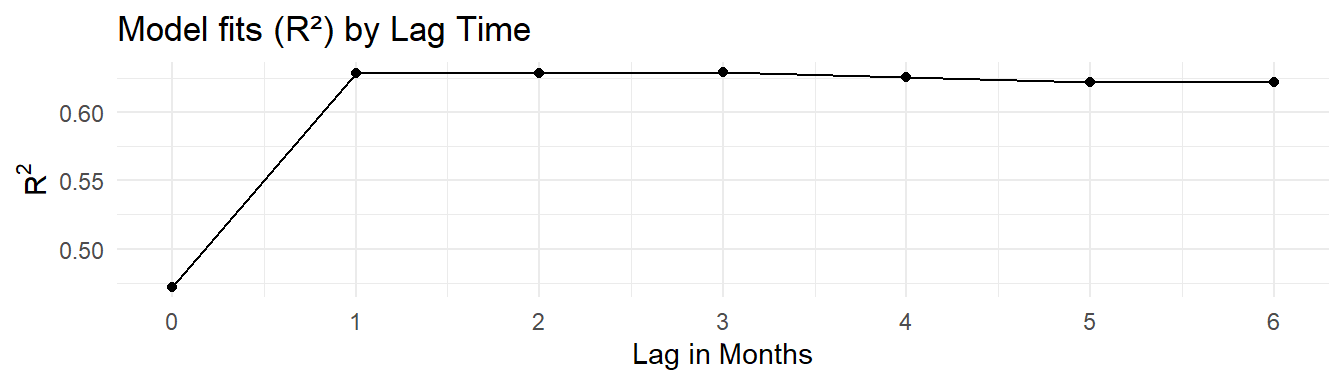
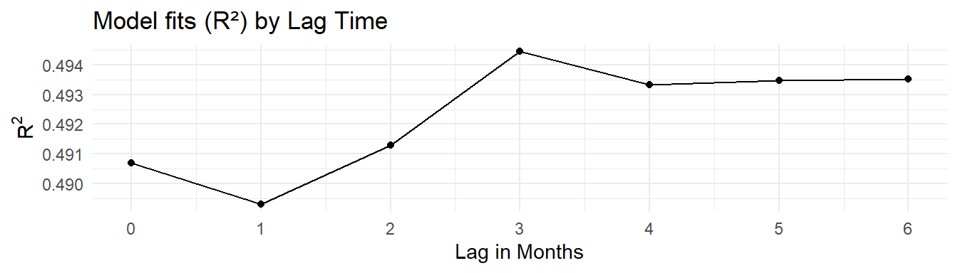
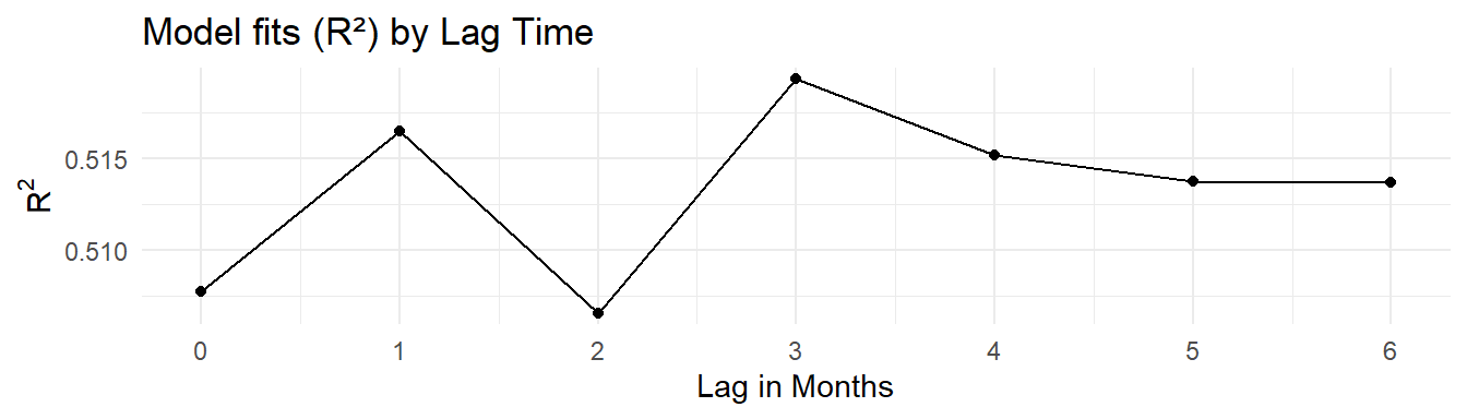
where the coefficients \(\beta_2\) and \(\beta_3\) represent the influence of salinity and temperature on chlorophyll-a concentrations. Chlorophyll is modelled using a log-normal distribution (using a GLM with a log-link function) to better capture extreme values and loading is also log-transformed. Below shows the explained deviance (pseudo-r-squared for GLMs) for each cumulative lag model.
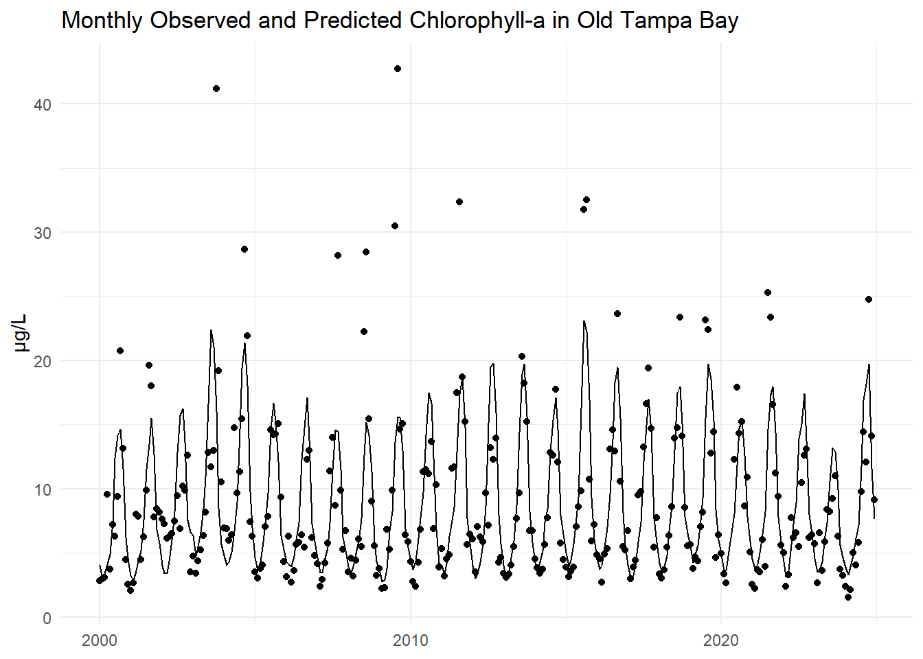
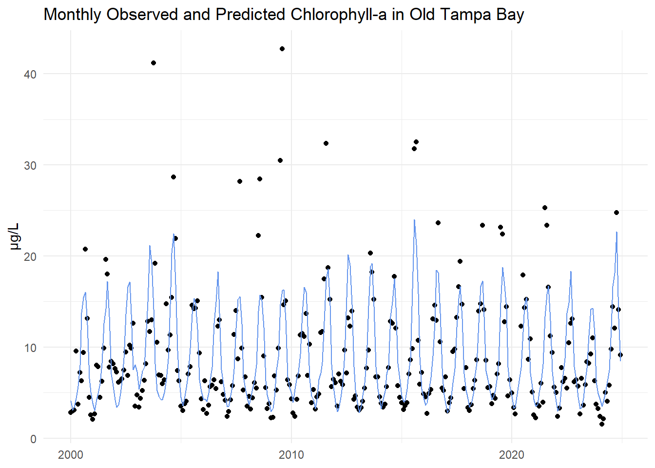
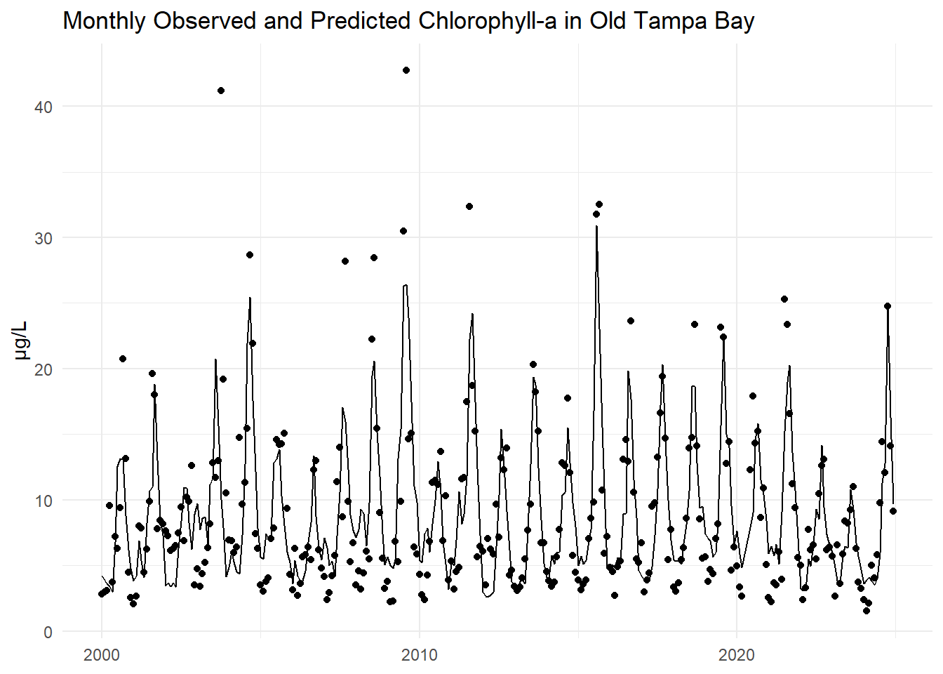
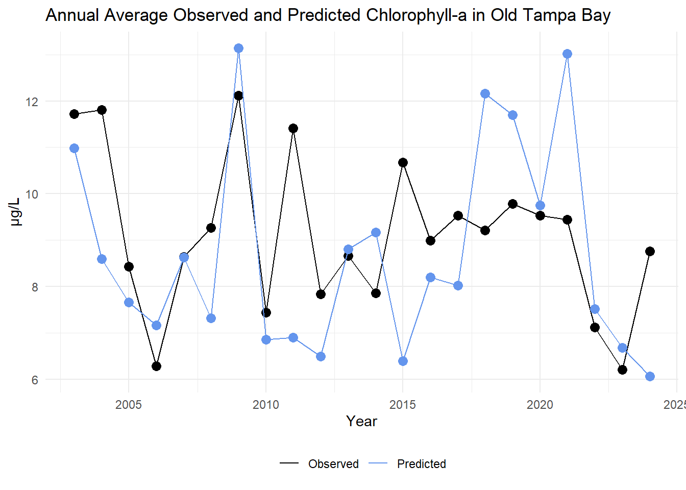
The model with a lag of 3 months for loading was used below. The monthly observed and predicted chlorophyll-a concentrations are compared for Old Tampa Bay below.
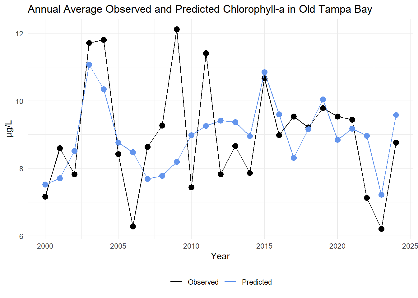
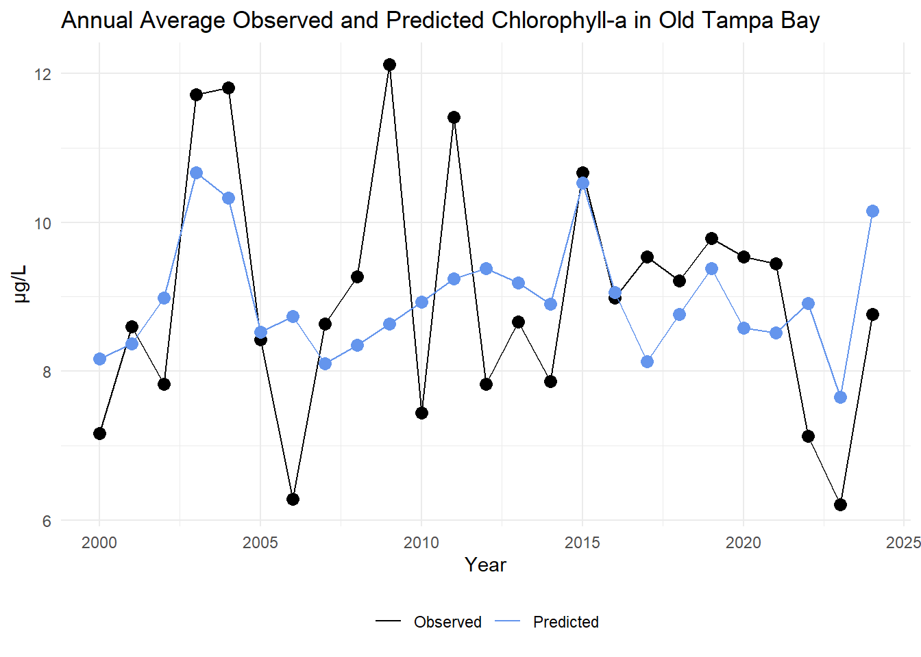
The annual average observed and predicted chlorophyll-a concentrations are compared for Old Tampa Bay below.

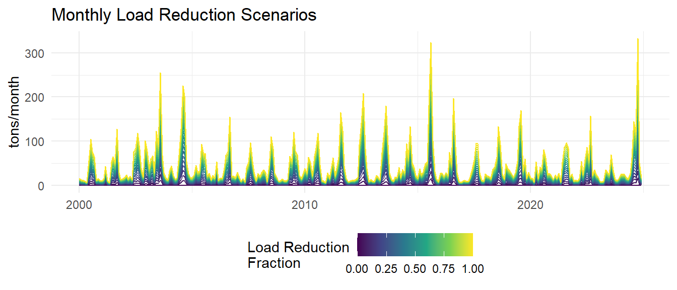
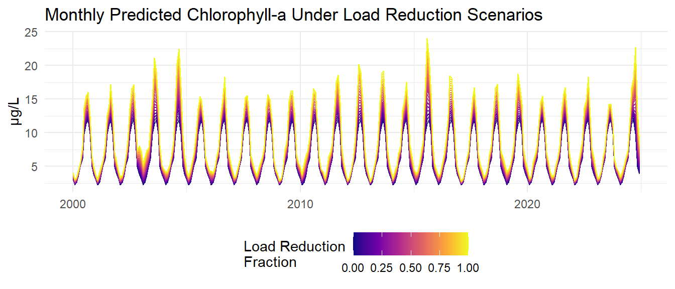
Monthly and annual model predictions are then generated for various nitrogen load reduction scenarios using the new log-model with additional predictors. Monthly loads are reduced by fractions ranging from 5% to 100% in 5% increments. The models are then used to predict chlorophyll-a concentrations under each load reduction scenario.
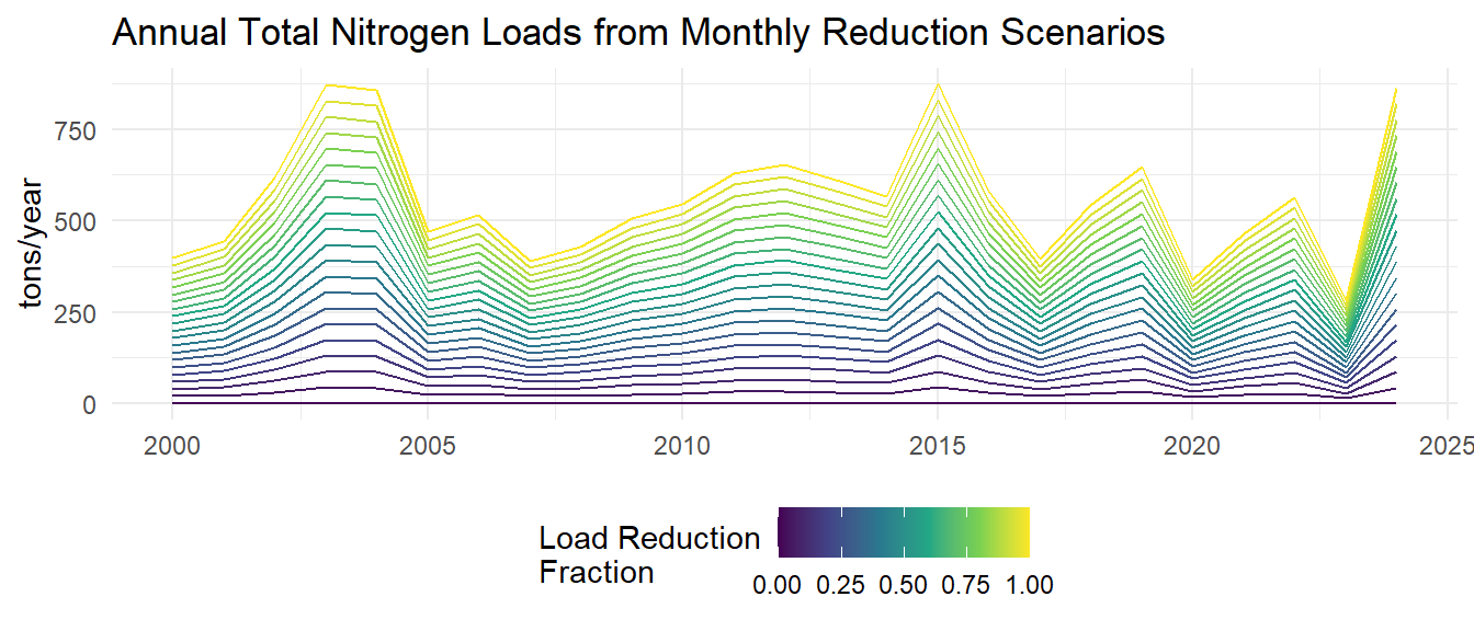
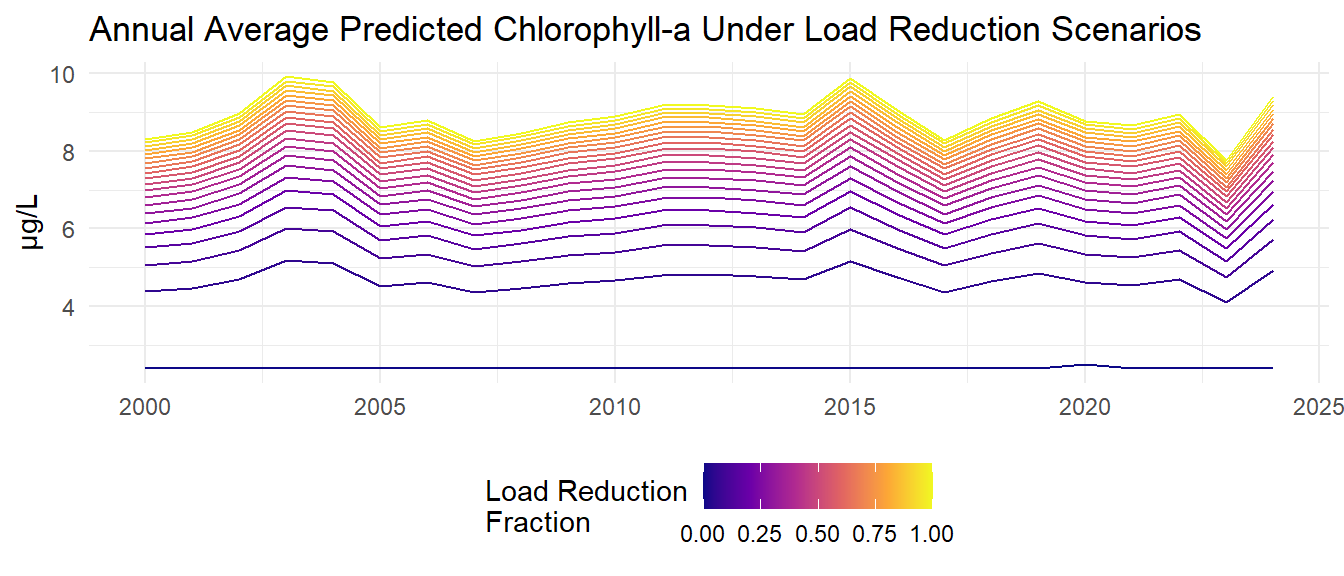
Monthly total nitrogen loads are then summed for the annual nitrogen loads and model predictions are aggregated to the annual average predicted chlorophyll-a concentration for each load reduction scenario.

Annual load estimates and chlorophyll-a predictions for each load reduction scenario are then averaged across the years.
Plotting these averages against each other can demonstrate an expected response of chlorophyll to load changes for the model. The plot below shows each point as the average predicted chlorophyll-a versus the average total nitrogen load for each load reduction scenario. The dashed red line indicates the target chlorophyll-a concentration of 8.5 µg/L. The arrow indicates the estimated nitrogen load needed to achieve the target chlorophyll-a concentration based on linear interpolation of the average response curves. The estimated load needed to achieve 8.5 µg/L chlorophyll-a is 439 tons/year.
Model 3: Load Response by Year
A final model structure was evaluated that let the load response vary by year. Only year and load were used as the predictors (month was removed).
\[ \text{chla}_{t} = \beta_1 \left( \Sigma_{i = I_0}^{I_n} L_{t - i} \right) + \beta_2 year_v \left( \Sigma_{i = I_0}^{I_n} L_{t - i} \right) \]
where \(year_v \left( \Sigma_{i = I_0}^{I_n} L_{t - i} \right)\) is an interaction term between year (as a factor) and the cumulative load evaluated at different lags from \(I_0\) for the present month to \(I_n\) months.
The model with a lag of 3 months for loading was used below. The monthly observed and predicted chlorophyll-a concentrations are compared for Old Tampa Bay below.

The annual average observed and predicted chlorophyll-a concentrations are compared for Old Tampa Bay below.

Monthly and annual model predictions are then generated for various nitrogen load reduction scenarios using the new model where the chlorophyll response to loading varies between years. Monthly loads are reduced by fractions ranging from 5% to 100% in 5% increments. The models are then used to predict chlorophyll-a concentrations under each load reduction scenario.
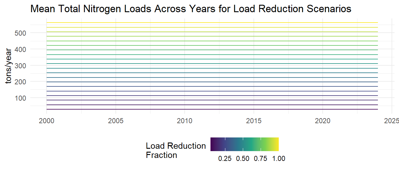
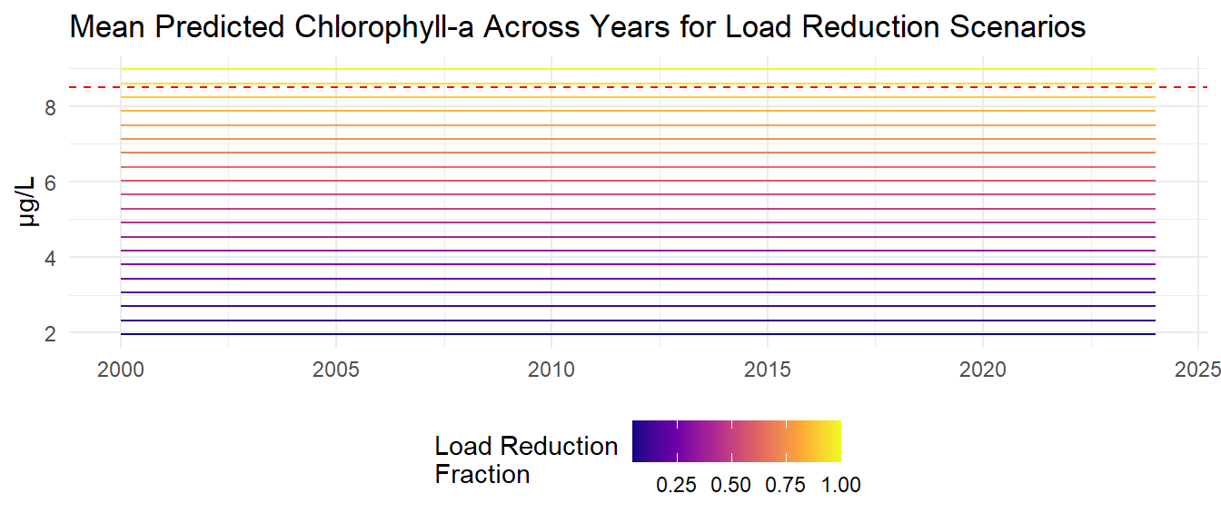
Monthly total nitrogen loads are then summed for the annual nitrogen loads and model predictions are aggregated to the annual average predicted chlorophyll-a concentrations for each load reduction scenario.
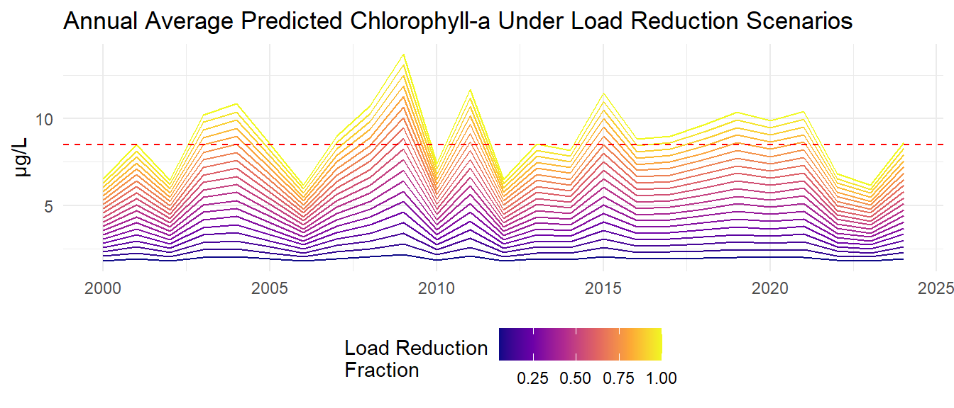
Annual load estimates and chlorophyll-a predictions for each load reduction scenario are then averaged across the years.
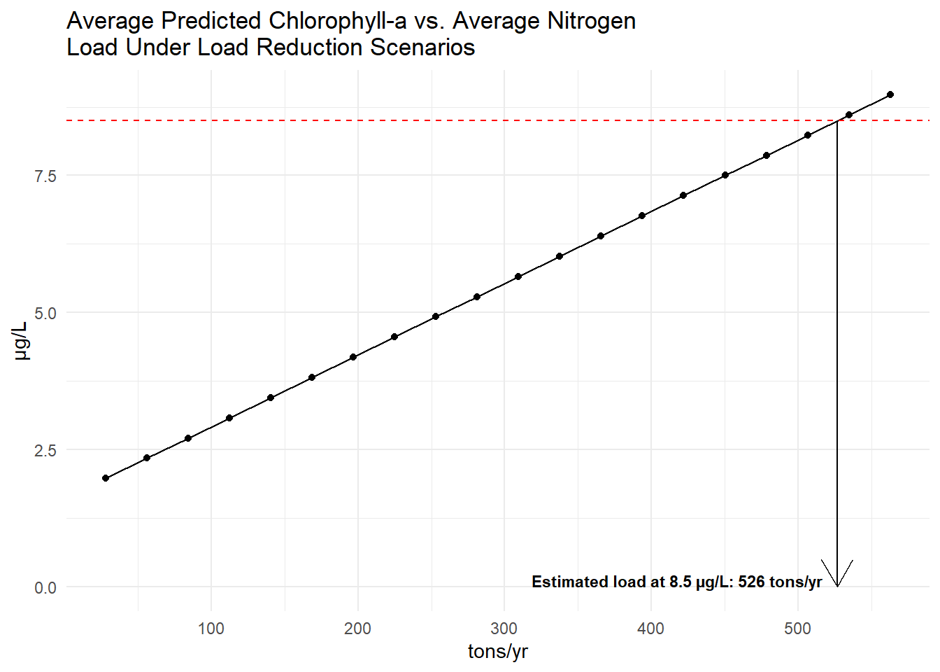
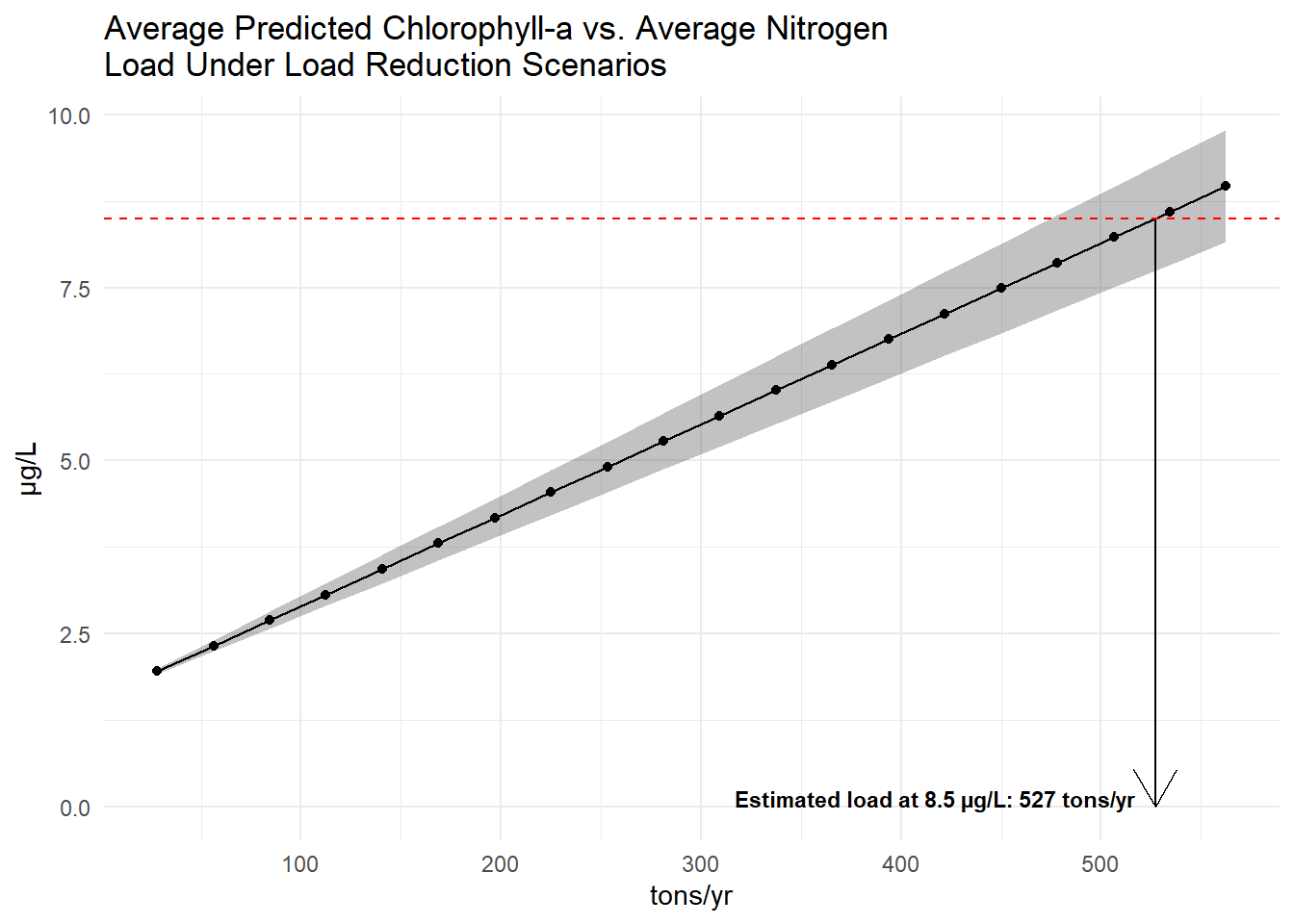
Plotting these averages against each other can demonstrate an expected response of chlorophyll to load changes for the model. The plot below shows each point as the average predicted chlorophyll-a versus the average total nitrogen load for each load reduction scenario. The dashed red line indicates the target chlorophyll-a concentration of 8.5 µg/L. The arrow indicates the estimated nitrogen load needed to achieve the target chlorophyll-a concentration based on linear interpolation of the average response curves. The estimated load needed to achieve 8.5 µg/L chlorophyll-a is 527 tons/year.
OTB Pinellas County Data
The above analyses for Old Tampa Bay were repeated using monitoring data from Pinellas County. Chlorophyll-a data (corrected for Pheophytin) are available from 2003 to present for the western side of Old Tampa Bay. The three models were evaluated to assess the potential loading associated with 8.5 \(\mu\)g/L of chlorophyll following similar methods as above. Only relevant plots and model summaries are shown below.
Model 1
\[ \text{chla}_{t} = \alpha_{t} + \beta \left( \Sigma_{i = I_0}^{I_n} L_{t - i} \right) \]
The estimated load needed to achieve 8.5 \(\mu\)g/L chlorophyll-a is 466 tons/year.
Model 2
\[ log_{10}\text{chla}_{t} = \alpha_{t} + \beta_1 log_{10}\left( \Sigma_{i = I_0}^{I_n} L_{t - i} \right) + \beta_2 \text{temp}_{t} \]
Note: Salinity excluded for better assocation of chlorophyll-a with loading.
The estimated load needed to achieve 8.5 \(\mu\)g/L chlorophyll-a is 464 tons/year.
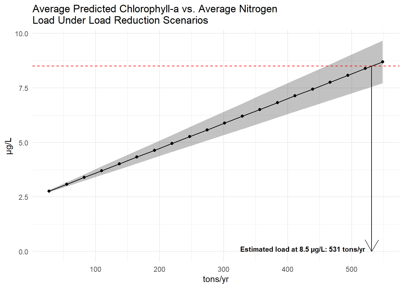
Model 3
\[ \text{chla}_{t} = \beta_1 \left( \Sigma_{i = I_0}^{I_n} L_{t - i} \right) + \beta_2 year_v \left( \Sigma_{i = I_0}^{I_n} L_{t - i} \right) \]
The estimated load needed to achieve 8.5 \(\mu\)g/L chlorophyll-a is 531 tons/year.
Summary Table
Dataset | Model 1: Original | Model 2: Log, Addl Predictors | Model 3: By Year |
|---|---|---|---|
EPC | 466 | 439 | 527 |
Pinellas | 466 | 464 | 531 |