This document provides some examples of the likelihood of obtaining the three TBNI action categories (stay the course, caution, on alert) based on seagrass cover. The intent is to understand potential targets for seagrass cover to obtain a desired TBNI outcome. Whether it does that is another question.
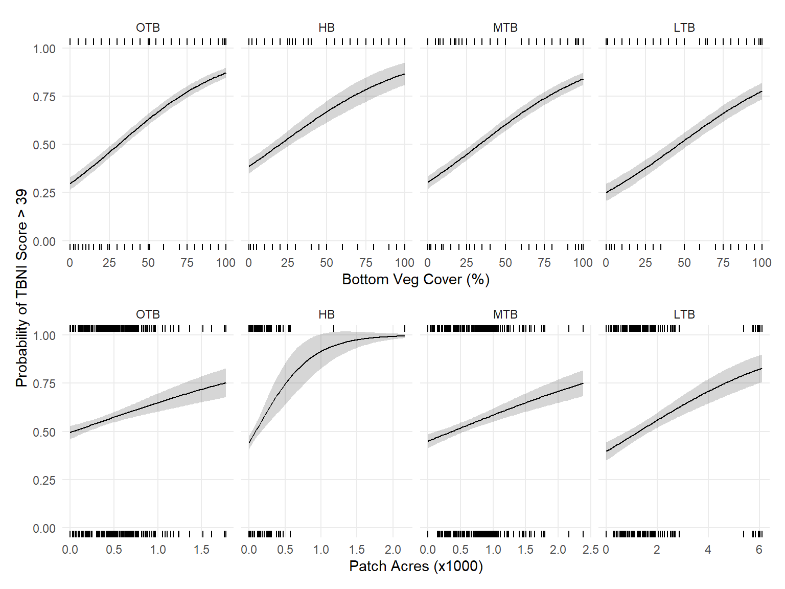
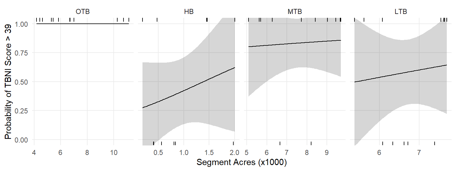
Likelihood of obtaining a TBNI score > 39 as the midpoint between all action categories based on seagrass cover from the FIM data or seagrass patch size from SWFWMD
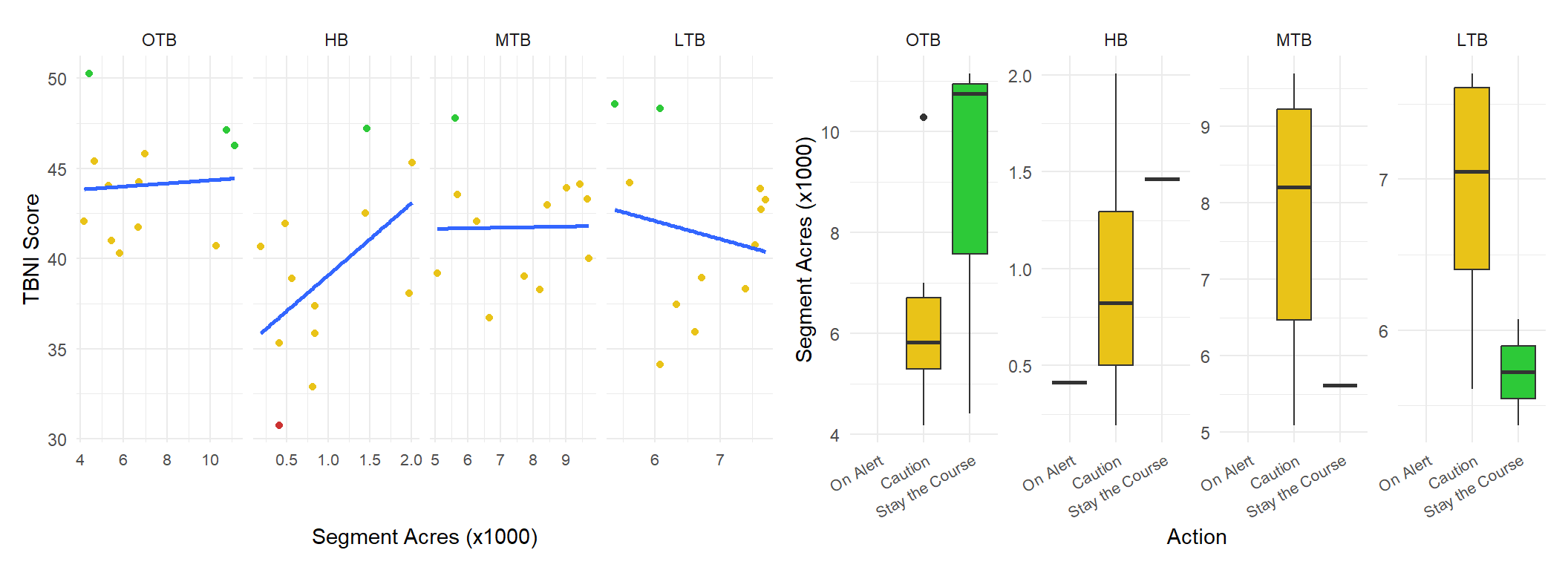
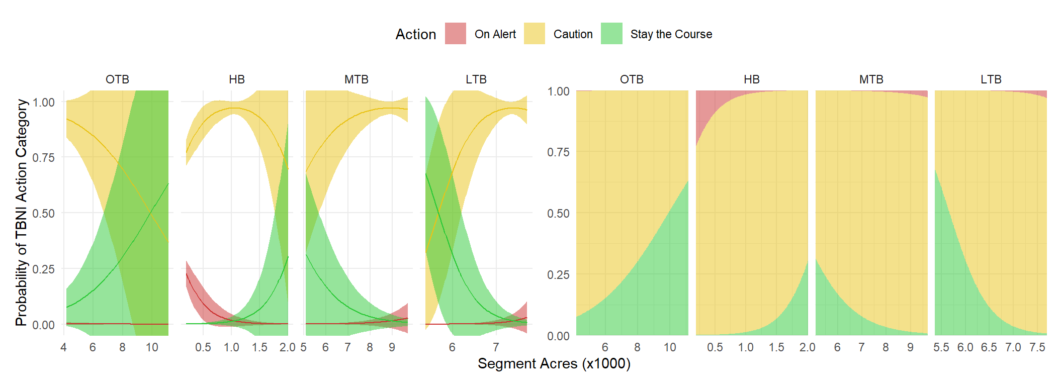
Likelihood of obtaining each of three TBNI action categories based on seagrass acreage by bay segment.
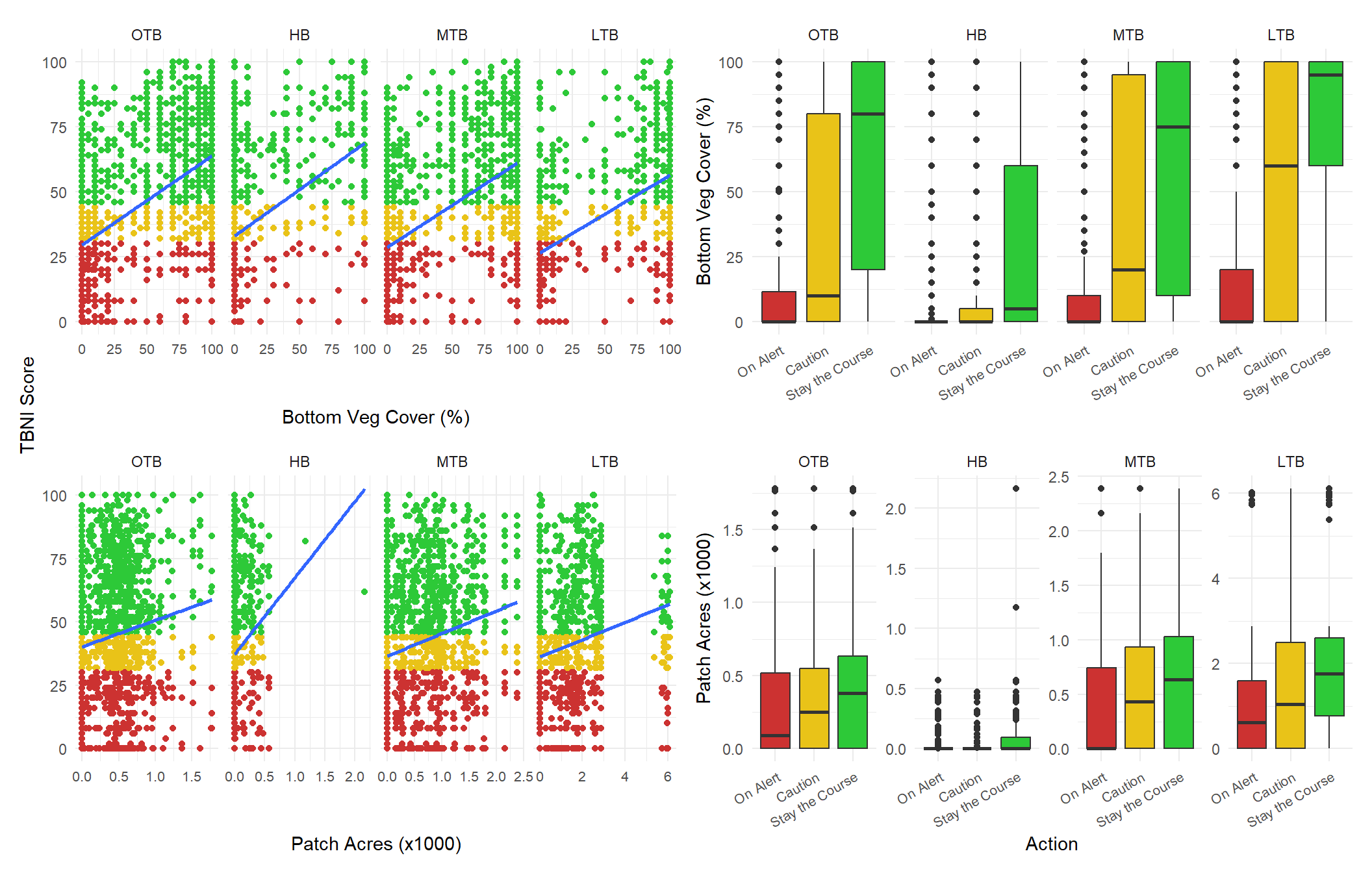
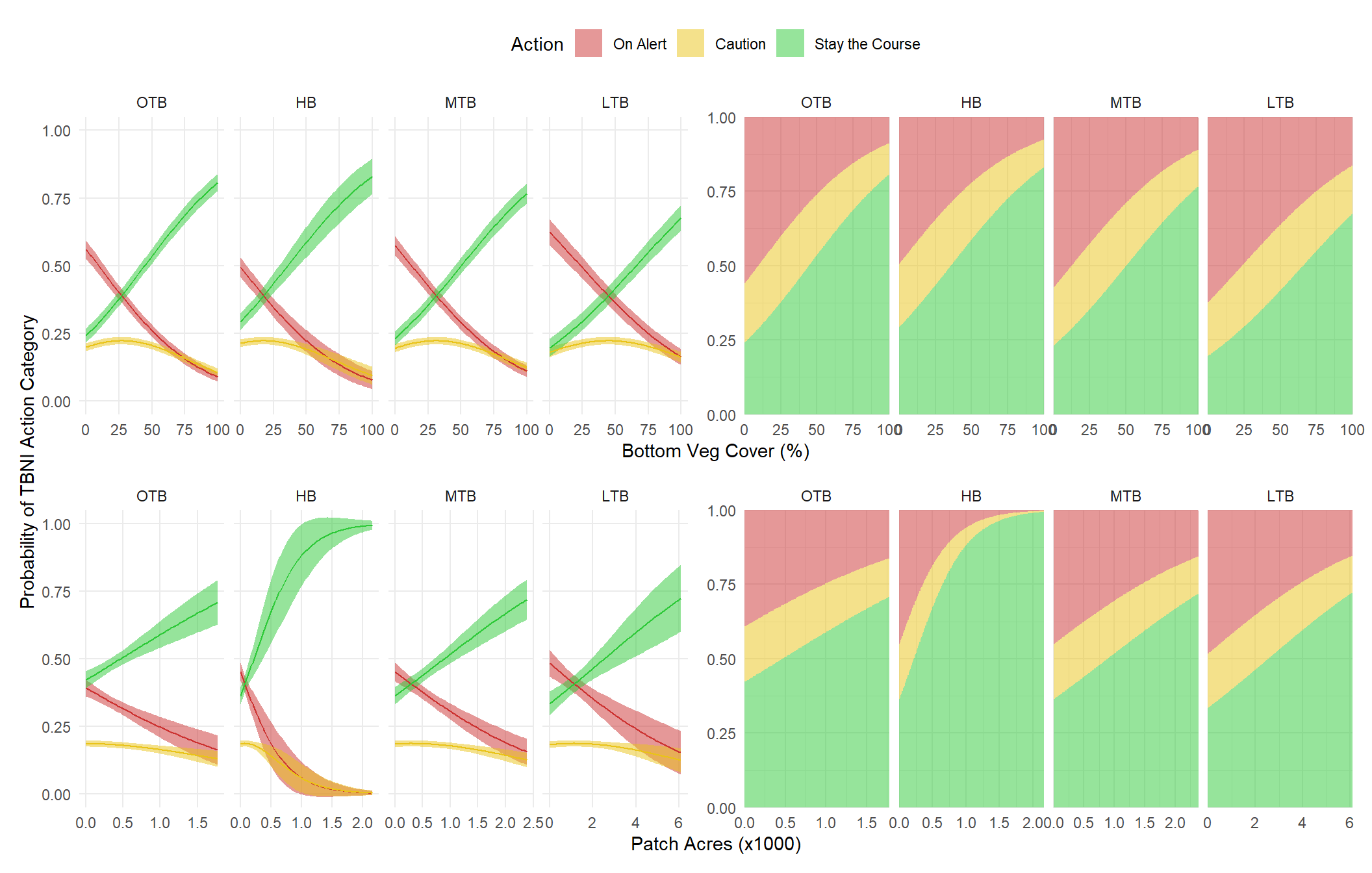
TBNI Action categories and scores compared to seagrass cover from the FIM data or seagrass patch size from SWFWMD.Likelihood of obtaining a TBNI score > 39 as the midpoint between all action categories based on seagrass cover from the FIM data or seagrass patch size from SWFWMDLikelihood of obtaining each of three TBNI action categories based on seagrass cover from the FIM data or seagrass patch size from SWFWMD.TBNI Action categories and scores compared to seagrass acreage by bay segmentLikelihood of obtaining a TBNI score > 39 as the midpoint between all action categories based on seagrass acreage by bay segmentLikelihood of obtaining each of three TBNI action categories based on seagrass acreage by bay segment.