Exploring 2024 TBNI results

library(tidyverse)
library(here)
library(patchwork)
library(sf)
library(leaflet)
library(tbeptools)

data(fimstations, package = 'tbeptools')
data(tbseg, package = 'tbeptools')

load(file = here('data/tbniscr.RData'))
load(file = here('data/sgdat2024.RData'))

hbsgdat <- sgdat2024 |> 
    filter(FLUCCSCODE %in% c(9113, 9116)) |> 
    st_transform(st_crs(fimstations)) |> 
    st_make_valid() |> 
    mutate(
        FLUCCSCODE = case_when(
            FLUCCSCODE == 9113 ~ 'Patchy',
            FLUCCSCODE == 9116 ~ 'Continuous'
        )
    )
hbsgdat <- hbsgdat[tbseg |> filter(bay_segment == 'HB'), ]

segshr <- c('OTB', 'HB', 'MTB', 'LTB')

hydrolab <- read.csv(url('https://github.com/tbep-tech/tbni-proc/raw/refs/heads/master/data/FIM_HydroLab_1996-2024.csv'))

bssize <- 13

yrs <- c(2022:2024)

# fim station salinity, temp
hydrodat <- hydrolab |> 
  filter(Depth == min(Depth), .by = c(Reference,  Year, Month)) |> 
  summarise(
    temp = mean(Temperature, na.rm = T),
    sal = mean(Salinity, na.rm = T),
    .by = c(Reference, Year, Month)
  )

#tbni by month, segment
tbnihydro <- tbniscr |> 
  rename(tbni = TBNI_Score) |> 
  left_join(hydrodat, by = c('Reference', 'Year', 'Month'))

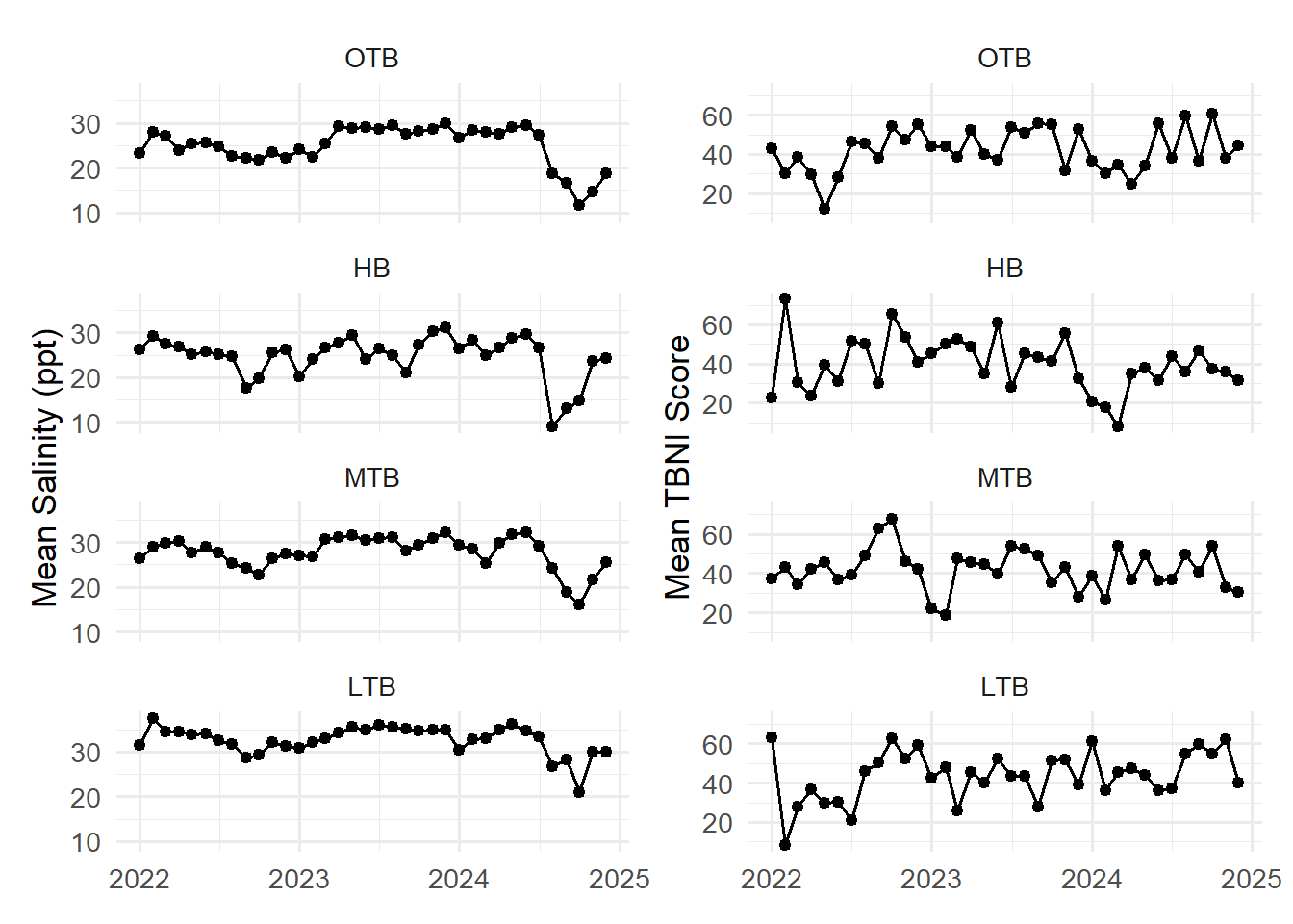
tbniscrsum <- tbnihydro |> 
  summarize(
    tbni = mean(tbni, na.rm = TRUE),
    sal = mean(sal, na.rm = TRUE),
    temp = mean(temp, na.rm = TRUE),
    Count = n(), 
    .by = c(Month, Year, bay_segment)
  ) |> 
  mutate(
    bay_segment = factor(bay_segment, levels = segshr), 
    date = as.Date(paste(Year, Month, "01", sep = "-"))
  )

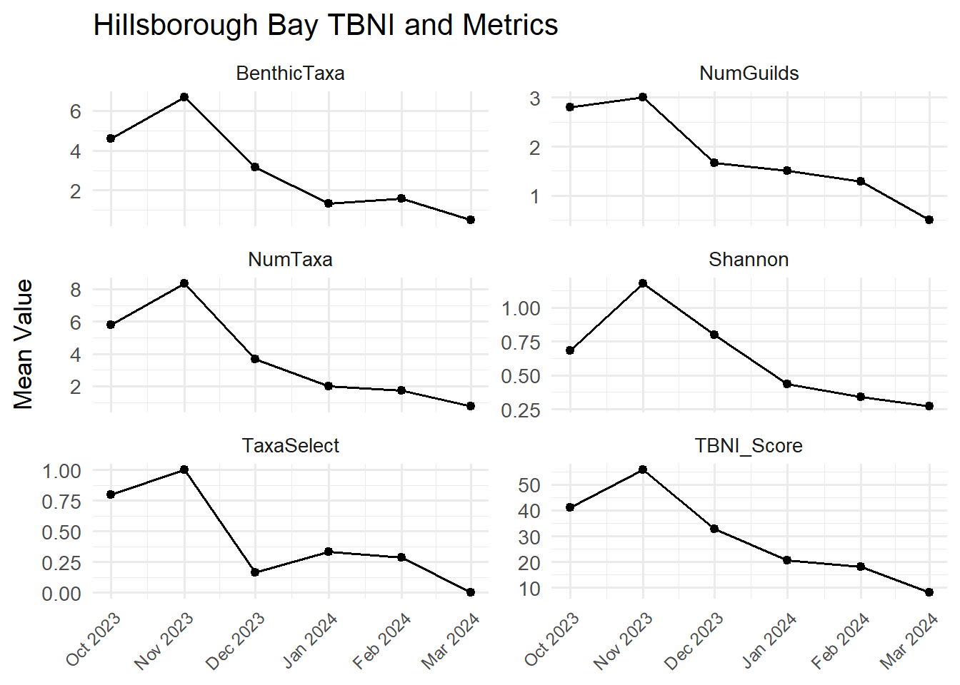
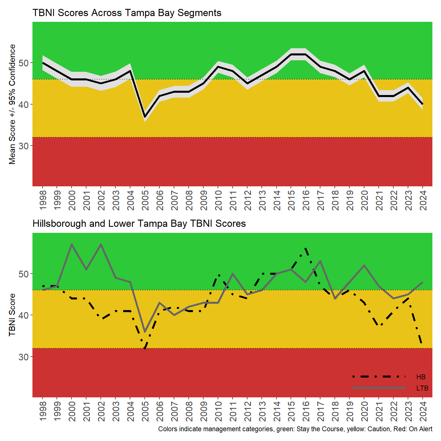
perc <- c(32, 46)
tomap <- tbniscr |> 
    mutate(date = as.Date(paste(Year, Month, "01", sep = "-"))) |>
    filter(date >= as.Date('2023-12-01') & date <= as.Date('2024-03-01')) |> 
    filter(bay_segment == 'HB') |> 
    mutate(
        Action = findInterval(TBNI_Score, perc),
        outcome = factor(Action, levels = c('0', '1', '2'), labels = c('red', 'yellow', 'green')),
        outcome = dplyr::case_when(
            outcome == 'green' ~ '#2DC938', 
            outcome == 'yellow' ~ '#E9C318', 
            outcome == 'red' ~ '#CC3231'
        )
    ) |> 
    select(Reference, date, TBNI_Score, outcome, NumTaxa)
tomap <- inner_join(fimstations |> select(-bay_segment), tomap, by = 'Reference')
bsmap <- tbeptools::util_map(tomap, minimap = NULL)

map_fun <- function(tomap, date, bsmap, hbsgdat, show_richness = FALSE){

    tomapdt <- tomap |> 
        mutate(
            radius_scaled = scales::rescale(NumTaxa, to = c(5, 18))
        ) |> 
        filter(date == !!date)
    
    # Create color palette function for FLUCCSCODE
    flucc_pal <- colorFactor(
        palette = c("#228B22", "#90EE90"),
        domain = c("Patchy", "Continuous")
    )
    
    # Set up circle marker parameters based on show_richness
    if (show_richness) {
        # Create color palette for richness
        richness_pal <- colorNumeric(
            palette = "Blues",
            domain = tomap$NumTaxa
        )
        
        circle_params <- list(
            fillColor = ~richness_pal(NumTaxa),
            radius = ~radius_scaled,
            label = ~paste0('Site ', Reference, ' (Richness: ', NumTaxa, ')')
        )
        
        # Add richness legend
        legend_richness <- TRUE
    } else {
        circle_params <- list(
            fillColor = ~outcome,
            radius = 5,
            label = ~paste0('Site ', Reference, ' (TBNI: ', round(TBNI_Score, 1), ')')
        )
        
        legend_richness <- FALSE
    }
    
    map_result <- bsmap |> 
        addPolygons(
            data = hbsgdat,
            fillColor = ~flucc_pal(FLUCCSCODE),
            fillOpacity = 0.7,
            weight = 0,       # border width
            opacity = 1
        ) |> 
        addCircleMarkers(
            data = tomapdt, 
            layerId = ~Reference,
            stroke = T,
            color = 'black',
            fill = TRUE,
            fillOpacity = 1,
            weight = 1, 
            fillColor = circle_params$fillColor,
            radius = circle_params$radius,
            label = circle_params$label
        ) |>
        addLegend(
            pal = flucc_pal,
            values = hbsgdat$FLUCCSCODE,
            title = "Seagrass",
            position = "bottomright",
            opacity = 1
        )
    
    # Add richness legend if needed
    if (legend_richness) {
        map_result <- map_result |>
            addLegend(
                pal = richness_pal,
                values = tomap$NumTaxa,
                title = "Total Richness",
                position = "topright",
                opacity = 1
            )
    }
    
    return(map_result)
}

Time series

TBNI and salinity

p1 <- ggplot(tbniscrsum |> filter(Year %in% yrs), aes(x = date, y = sal)) +
  geom_line() +
  geom_point() +
  facet_wrap(~ bay_segment, ncol = 1) +
  labs(
    x = NULL,
    y = "Mean Salinity (ppt)"
  ) +
  theme_minimal(base_size = bssize)

p2 <- ggplot(tbniscrsum |> filter(Year %in% yrs), aes(x = date, y = tbni)) +
  geom_line() +
  geom_point() +
  facet_wrap(~ bay_segment, ncol = 1) +
  labs(
    x = NULL,
    y = "Mean TBNI Score"
  ) +
  theme_minimal(base_size = bssize)

p1 + p2 + plot_layout(ncol = 2)

HB metrics and TBNI

toplo <- tbniscr |> 
  filter(Year %in% yrs) |> 
  select(-starts_with('Score')) |> 
  pivot_longer(
    cols = c(TBNI_Score, NumTaxa, BenthicTaxa, TaxaSelect, NumGuilds, Shannon),
    names_to = "Metric",
    values_to = "Value"
  ) |> 
  summarise(
    Value = mean(Value, na.rm = TRUE),
    .by = c(bay_segment, Year, Month, Metric)
  ) |> 
  mutate(
    segment = factor(bay_segment, levels = segshr), 
    date = as.Date(paste(Year, Month, "01", sep = "-"))
  ) |> 
  filter(bay_segment %in% 'HB' & date >= as.Date('2023-10-01') & date <= as.Date('2024-03-01'))

ggplot(toplo, aes(x = date, y = Value)) +
  geom_line() +
  geom_point() +
  scale_x_date(date_labels = "%b %Y") +
  facet_wrap(~ Metric, scales = 'free_y', ncol = 2) +
  labs(
    title = "Hillsborough Bay TBNI and Metrics",
    x = NULL,
    y = "Mean Value"
  ) +
  theme_minimal(base_size = bssize) + 
  theme(
    axis.text.x = element_text(angle = 45, hjust = 1, size = 9)
  )

Lagged salinity

Lagged salinity correlation

toest <- tbniscrsum |> 
    filter(Year %in% c(2020, 2021, yrs)) |> 
    crossing(
        lg = 0:24
    ) |> 
    group_nest(lg, bay_segment) |> 
    mutate(
        corv = purrr::pmap(list(lg, data), function(lg, data) {

            tocor <- data |> 
                arrange(Year, Month) |>
                mutate(
                    sallg = lag(sal, n = lg),
                ) |> 
                filter(Year > 2021)
            
            out <- cor.test(tocor$sallg, tocor$tbni)

            tibble(
                cor = out$estimate,
                pval = out$p.value
            )

        })
    ) |> 
    select(-data) |> 
    unnest(corv) |> 
    mutate(
        pval = ifelse(pval < 0.05, '*', 'ns'), 
        bay_segment = factor(bay_segment, levels = segshr)
    )

ggplot(toest, aes(x = lg, y = cor, fill = pval)) +
    geom_col(color = 'black') +
    scale_fill_manual(values = c('grey', 'white')) +
    facet_wrap(~ bay_segment, ncol = 1) +
    labs(
        title = "Correlation of TBNI with Lagged Salinity",
        subtitle = '2022 - 2024',
        x = "Salnity Lag (months prior)",
        y = "Correlation Coefficient",
        fill = "p-value"
    ) +
    theme_minimal(base_size = bssize) + 
    theme(
        legend.position = 'top'
    )

Lagged salinity scatter

toest <- tbniscrsum |> 
    filter(Year %in% c(2020, 2021, yrs)) |> 
    arrange(bay_segment, Year, Month) |>
    mutate(
        sallg = lag(sal, n = 23), 
        .by = bay_segment
    ) |> 
    filter(Year > 2021) |>
    mutate(
        bay_segment = factor(bay_segment, levels = segshr)
    )

ggplot(toest, aes(x = sallg, y = tbni)) +
    geom_text(aes(color = factor(Year), label = Month)) +
    geom_smooth(method = 'lm', se = T, color = 'black') +
    facet_wrap(~ bay_segment, ncol = 2) +
    labs(
        title = "Correlation of TBNI with Lagged Salinity (Hillsborough Bay)",
        subtitle = '2022 - 2024',
        x = "Salinity 23 Months Prior (ppt)",
        y = "Monthly TBNI Score", 
        color  = 'Year'
    ) +
    theme_minimal(base_size = bssize) + 
    theme(
        legend.position = 'top'
    )

TBNI scores by month

Dec 2023

map_fun(tomap, as.Date('2023-12-01'), bsmap, hbsgdat)

Jan 2024

map_fun(tomap, as.Date('2024-01-01'), bsmap, hbsgdat)

Feb 2024

map_fun(tomap, as.Date('2024-02-01'), bsmap, hbsgdat)

Mar 2024

map_fun(tomap, as.Date('2024-03-01'), bsmap, hbsgdat)

Richness by month

Dec 2023

map_fun(tomap, as.Date('2023-12-01'), bsmap, hbsgdat, show_richness = TRUE)

Jan 2024

map_fun(tomap, as.Date('2024-01-01'), bsmap, hbsgdat, show_richness = TRUE)

Feb 2024

map_fun(tomap, as.Date('2024-02-01'), bsmap, hbsgdat, show_richness = TRUE)

Mar 2024

map_fun(tomap, as.Date('2024-03-01'), bsmap, hbsgdat, show_richness = TRUE)

Key Messages Graphic

tbniscr <- anlz_tbniscr(fimdata)
p1 <- show_tbniscrall(tbniscr) + 
    scale_y_continuous('Mean Score +/- 95% Confidence', limits = c(22, 58)) +
    labs(
        title = "TBNI Scores Across Tampa Bay Segments"
    )
p2 <- show_tbniscr(tbniscr, bay_segment = c('HB', 'LTB')) +
    scale_y_continuous('TBNI Score', limits = c(22, 58)) +
    labs(
        title = "Hillsborough and Lower Tampa Bay TBNI Scores",
        caption = 'Colors indicate management categories, green: Stay the Course, yellow: Caution, Red: On Alert'
    )

p1 / p2 + plot_layout(ncol = 1)