Exploratory analysis: 2023 data

Author

Affiliation

Marcus Beck, mbeck@tbep.org, Sheila Scolaro, sscolaro@tbep.org

Tampa Bay Estuary Program

Published

August 6, 2024

Code

library(tidyverse)
library(sf)
library(mapview)
library(here)
library(tbeptools)
library(patchwork)
library(hrbrthemes)

load(file = here('data/metadat.RData'))
load(file = here('data/tempdat.RData'))
load(file = here('data/otbsub.RData'))

sublevs <- c('NW', 'NE', 'CW', 'CE', 'SW', 'SE')

# remote metadat extra columns
metastrip <- metadat %>% 
  select(-site, -logger, -yr) %>% 
  st_set_geometry(NULL)

# combine temp and meta, remove bartow outlier
dat <- tempdat %>% 
  left_join(metastrip, by = 'yr_site_logger') %>% 
  filter(!site %in% '3SWB3') %>% 
  filter(yr == 2023) %>%
  mutate(
    hr = hour(datetime),
    mo = month(deploy_date), 
    subseg = substr(site, 2, 3),
    subseg = factor(subseg, levels = sublevs), 
    side = case_when(
      grepl('W$', subseg) ~ 'West', 
      grepl('E$', subseg) ~ 'East'
    ), 
    side = factor(side, levels = c('West', 'East')),
    stratum = case_when(
      stratum == 'GAIN' ~ 'SEAGRASS', 
      stratum == 'LOSS' ~ 'BARE', 
      T ~ stratum
    )
  )

# baseline data
bsdat <- epcdata %>% 
  filter(bay_segment == 'OTB') %>% 
  filter(yr >= 2004 & yr <= 2018) %>% 
  # filter(mo %in% dat$mo) %>% 
  select(
    epchc_station, 
    SampleTime, 
    yr, 
    mo, 
    tempc = Temp_Water_Bottom_degC,
    lat = Latitude, 
    lon = Longitude
    ) %>% 
  st_as_sf(coords = c('lon', 'lat'), remove = F, crs = 4326) %>% 
  st_intersection(otbsub) %>% 
  mutate(
    subseg = factor(subseg, levels = sublevs)
  )

Background and questions

This document provides exploratory data analyses for the temperature logger deployments in Old Tampa Bay (OTB). The graphs herein are meant to provide initial quantitative support to address the following questions:

Are there differences in temperature at sites where seagrasses were lost compared to where it was gained?
Are these differences related to location in OTB, such that thermal stress may be higher along a spatial gradient (e.g., in relation to subembayments where hydrology as affected by land bridges)?

The questions follow the general hypothesis that seagrass loss in OTB could partially be explained by thermal stress, where seasonal temperature increases in recent years could stress seagrasses beyond their thermal maxima.

Confounding factors

The potential confounding effects of the following must be considered if the logger data are to be used to refute or support the hypothesis:

Temperature may differ given time of year or preceding weather, such that direct comparisons of data between deployment dates (and years) is not possible with the raw data, to address:
- Only compare within deployment dates
- Or normalize the data across deployment dates, e.g., subtract the mean temperature for each deployment date
Within and between deployment dates, overall temperature may vary by location. Although we are concerned that thermal stress may vary spatially, any comparison to historical data must account for natural spatial patterns in temperature in addition to potential recent increases in temperature regardless of location.
Any statistical test must account for temporal correlation in the continuous monitoring data:
- Summary or subsets of the data can be evaluated (e.g, daily maxima)
- Or individual time series can be detrended to remove natural diurnal variation (Fourier transform or some other filter)

Sample locations

This map shows the OTB sub-segments, long-term EPC monitoring stations (red), and sites for the current project (blue).

Code

tomap1 <- bsdat %>% 
  select(epchc_station) %>% 
  unique()
mapview(otbsub, zcol = NULL, layer.name = 'Sub-segments', col.regions = 'lightblue', homebutton = F, legend = F, map.types = 'CartoDB.Positron') + 
  mapview(tomap1, alpha = 0, layer.name = 'EPC long-term', homebutton = F, col.regions = 'red', legend = F) + 
  mapview(metadat, layer.name = 'Current project', homebutton = F)

Historical patterns

Long-term data from EPC were used to plot the range of values for bottom water temperatures, grouped by the OTB sub-segments. The horizontal lines are the medians and the points are colored by those that are in the same deployment months for the current project and those that are not. These data can be used as comparison with those from the current project.

Code

toplo <- bsdat %>% 
  st_set_geometry(NULL) %>% 
  mutate(
    tempmed = median(tempc, na.rm = T), 
    .by  = subseg, 
    julmo = ifelse(mo %in% unique(dat$mo), 'Deployment\nmonths', 'All other')
  ) 
ggplot(toplo, aes(x = subseg, y = tempc, group = subseg)) + 
  geom_point(aes(fill = julmo), position = position_dodge2(width = 0.4), alpha = 0.7, pch = 21, color  = "#FFFFFF00", size = 3) + 
  geom_boxplot(aes(y = tempmed, color = tempmed)) + 
  scale_color_distiller(palette = 'Reds', direction = 1) + 
  scale_fill_manual(values = c('black', 'green')) + 
  theme(
    panel.grid.minor = element_blank(), 
    panel.grid.major.x = element_blank()
  ) +
  guides(fill = guide_legend(reverse = T)) +
  labs(
    x = NULL, 
    y = 'Bottom temp (C)', 
    color = 'Median', 
    fill = 'Month',
    title = 'EPC 2004-2018 montly bottom temperature'
  )

Initial summary graphs

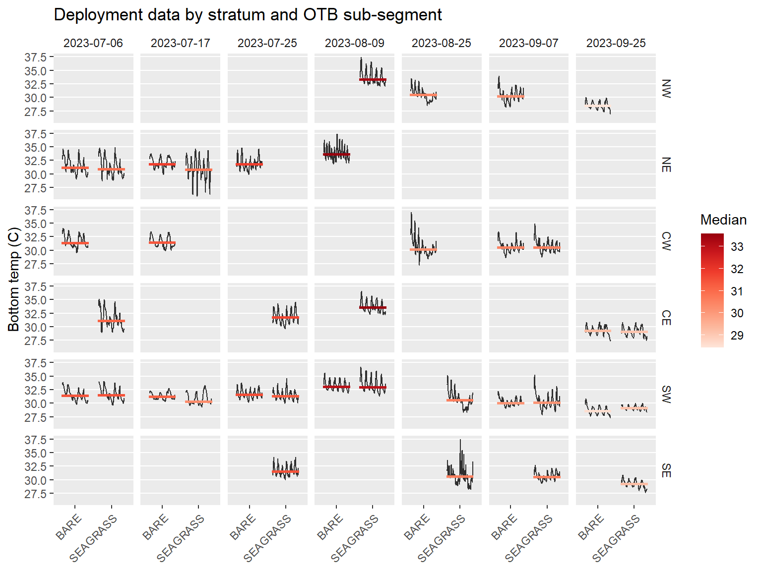
All data for the current project can be viewed in the same plot that shows the individual time series by deployment date, stratum, and OTB sub-segment.

Code

toplo <- dat %>% 
  mutate(
    tempmed = median(tempc, na.rm = T), 
    .by  = c('subseg', 'deploy_date', 'stratum')
  ) 
ggplot(toplo, aes(x = stratum, y = tempc)) + 
  geom_line(position = position_dodge2(width = 0.7), alpha = 0.8, size = 0.5) + 
  facet_grid(subseg ~ deploy_date) +
  geom_boxplot(aes(y = tempmed, color = tempmed)) + 
  scale_color_distiller(palette = 'Reds', direction = 1) + 
  scale_fill_manual(values = c('black', 'green')) + 
  theme(
    panel.grid.minor = element_blank(), 
    panel.grid.major.x = element_blank(), 
    strip.background = element_blank(), 
    axis.text.x = element_text(angle = 45, hjust = 1)
  ) +
  labs(
    x = NULL, 
    y = 'Bottom temp (C)', 
    color = 'Median', 
    fill = 'Month',
    title = 'Deployment data by stratum and OTB sub-segment'
  )

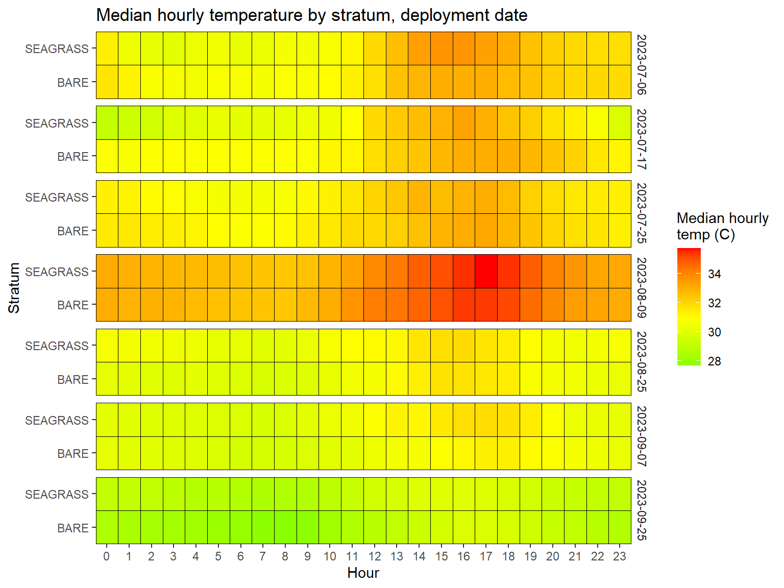
Additionally, a comparison of the median hourly temperatures for the data summarized by deployment date and stratum shows the diurnal range of values.

Code

toplo <- dat %>% 
  summarise(
    tempc = median(tempc, na.rm = T), 
    .by  = c('hr', 'deploy_date', 'stratum')
  ) 
ggplot(toplo, aes(x = hr, y = stratum, fill = tempc)) + 
  geom_tile(color = 'black') + 
  scale_fill_gradient2(low = 'green', mid = 'yellow', high = 'red', na.value = 'white', midpoint = median(toplo$tempc)) +
  scale_x_continuous(expand = c(0, 0), breaks = unique(toplo$hr)) + 
  scale_y_discrete(expand = c(0, 0)) +
  facet_grid(deploy_date ~ ., scales = 'free') +
  theme(
    strip.background = element_blank()
  ) + 
  labs(
    x = "Hour", 
    fill = "Median hourly\ntemp (C)", 
    y = 'Stratum', 
    title = 'Median hourly temperature by stratum, deployment date'
  )

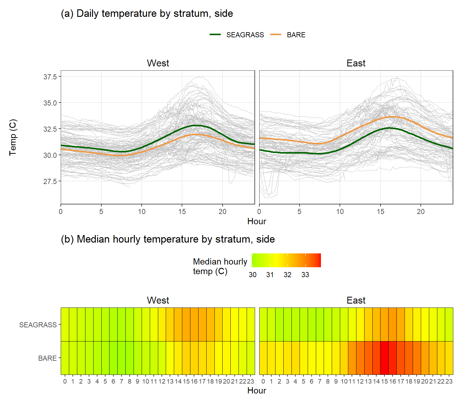
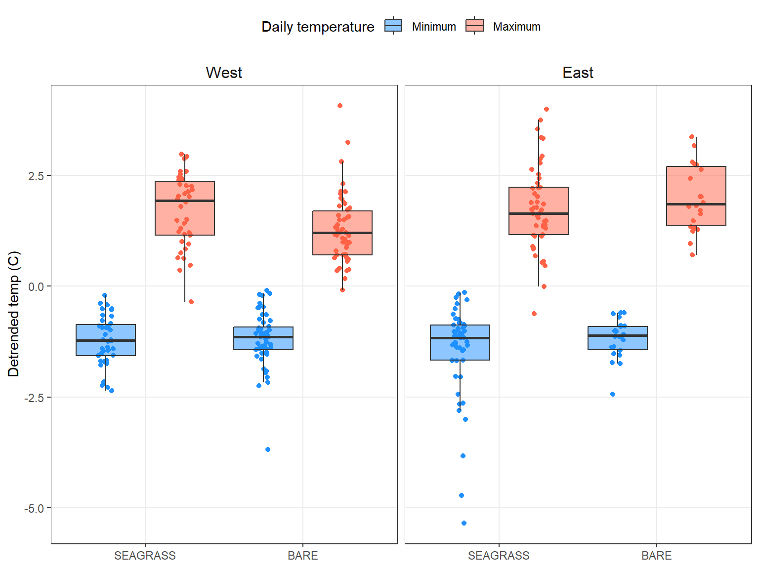
The daily data can also be evaluated relative to western or eastern stations in Old Tampa Bay.

Code

toplo <- dat %>% 
  mutate(
    date = date(datetime),
    min = minute(datetime) / 60,
    hrmin = hr + min,
    stratum = factor(stratum, levels = c('SEAGRASS', 'BARE'))
  ) %>% 
  unite('grp', date, site) %>% 
  mutate(
    n = n(), 
    .by = c('grp')
  )

p1 <- ggplot(toplo, aes(x = hrmin, y = tempc)) + 
  geom_line(aes(group = grp), linewidth = 0.25, color = 'grey') + 
  facet_grid( ~ side) +
  scale_color_manual(values = c('darkgreen', 'tan2')) +
  scale_x_continuous(expand = c(0, 0)) +
  geom_smooth(aes(color = stratum), se = F) +
  theme_bw() +
  theme(
    strip.background = element_blank(), 
    panel.grid.minor = element_blank(), 
    legend.position = 'top', 
    strip.text = element_text(size = 12)
  ) + 
  labs(
    x = "Hour", 
    y = 'Temp (C)',
    color = NULL,
    title = '(a) Daily temperature by stratum, side'
  )

toplo <- dat %>% 
  summarise(
    tempc = median(tempc, na.rm = T), 
    .by  = c('hr', 'side', 'stratum')
  ) 
p2 <- ggplot(toplo, aes(x = hr, y = stratum, fill = tempc)) + 
  geom_tile(color = 'black') + 
  scale_fill_gradient2(low = 'green', mid = 'yellow', high = 'red', na.value = 'white', midpoint = median(toplo$tempc)) +
  scale_x_continuous(expand = c(0, 0), breaks = unique(toplo$hr)) + 
  scale_y_discrete(expand = c(0, 0)) +
  facet_wrap(~side) +
  theme(
    strip.background = element_blank(), 
    strip.text = element_text(size = 12), 
    legend.position = 'top', 
    axis.text.x = element_text(size = 8)
  ) + 
  labs(
    x = "Hour", 
    fill = "Median hourly\ntemp (C)", 
    y = NULL, 
    title = '(b) Median hourly temperature by stratum, side'
  )

p1 + p2 + plot_layout(ncol = 1, heights = c(1, 0.5))

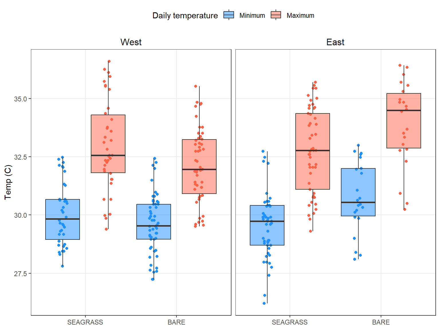
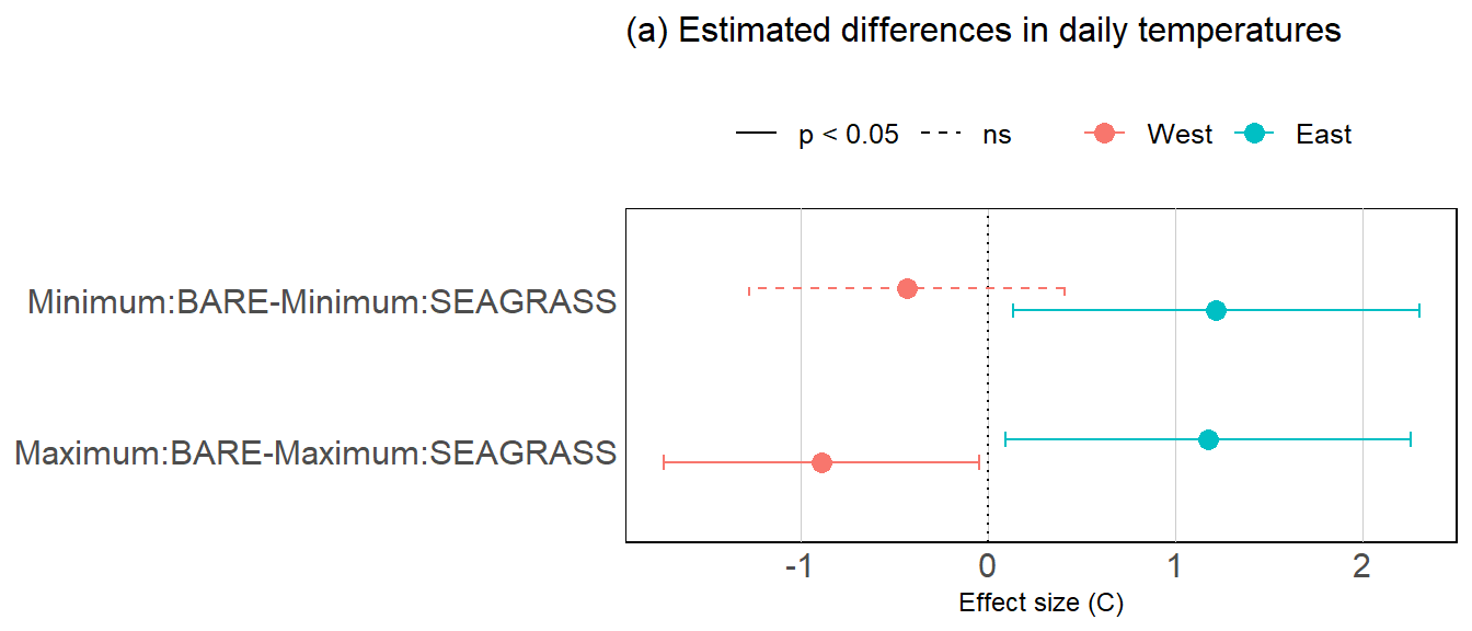
A more detailed evaluation of minimum and maximum daily temperatures again shows differences in east vs west locations. Days with incomplete observations were removed from this analysis.

Code

toplo <- dat %>% 
  mutate(
    date = date(datetime),
    stratum = factor(stratum, levels = c('SEAGRASS', 'BARE'))
  ) %>% 
  unite('grp', date, site) %>% 
  mutate(
    n = n(), 
    .by = c('grp')
  ) %>% 
  filter(n == 144) %>% 
  summarise(
    minv = min(tempc), 
    maxv = max(tempc), 
    .by = c(grp, stratum, side)
  ) %>% 
  pivot_longer(names_to = 'met', values_to = 'tempc', minv:maxv) %>% 
  mutate(
    met = factor(met, levels = c('minv', 'maxv'), labels = c('Minimum', 'Maximum'))
  )

metcol <- c('dodgerblue', 'tomato1')
wd <- 1
p <- ggplot(toplo, aes(x = stratum, y = tempc, fill = met)) +
  geom_point(aes(color = met), position = position_jitterdodge(dodge.width = wd, jitter.width = 0.2), show.legend = F) +
  geom_boxplot(position = position_dodge(width = wd), outlier.colour = NA, alpha = 0.5) +
  scale_color_manual(values = metcol) + 
  scale_fill_manual(values = metcol) +
  facet_grid(~side) +
  theme_bw() +
  theme(
    strip.background = element_blank(), 
    panel.grid.minor = element_blank(), 
    legend.position = 'top', 
    strip.text = element_text(size = 12)
  ) + 
  labs(
    y = 'Temp (C)', 
    x = NULL, 
    fill = 'Daily temperature'
  )
p

This plot shows the estimated differences in the daily minimum or maximum temperatures between seagrass and bare habitats, separated by east/west sides of Old Tampa Bay.

Code

sidemod <- toplo %>% 
  group_nest(side) %>% 
  mutate(
    mod = purrr::map(data, ~TukeyHSD(aov(tempc ~ met * stratum, data = .x)))
  )

toplo <- sidemod %>% 
  mutate(
    mod = purrr::map(mod, function(x){
      x$`met:stratum` %>% 
        data.frame %>% 
        mutate(
          comp = row.names(.)
        )
    })
  ) %>% 
  select(side, mod) %>% 
  unnest('mod') %>% 
  filter(comp %in% c("Minimum:BARE-Minimum:SEAGRASS", 
                     "Maximum:BARE-Maximum:SEAGRASS")
  ) %>% 
  mutate(
    pcol = ifelse(p.adj <= 0.05, 'p < 0.05', 'ns'), 
    pcol = factor(pcol, levels = c('p < 0.05', 'ns'))
  ) 

p <- ggplot(toplo, aes(y = comp, x = diff, linetype = pcol, col = side)) + 
  geom_vline(xintercept = 0, color = 'black', linetype = 'dotted') +
  geom_point(position = position_dodge(width = 0.3), size = 3) + 
  geom_errorbar(aes(xmin = lwr, xmax = upr), position = position_dodge(width = 0.3), width = 0.2) + 
  scale_linetype_manual(values = c('solid', 'dashed'), drop = F) +
  theme_ipsum(plot_margin = margin(5, 5, 5, 5)) + 
  theme(
    strip.placement = 'outside',
    panel.grid.minor = element_blank(),
    panel.grid.major.y = element_blank(),
    strip.background = element_blank(), 
    axis.title.y = element_blank(), 
    legend.title = element_blank(), 
    legend.position = 'top',
    axis.title.x = element_text(hjust = 0.5),
    strip.text.x = element_text(hjust = 0.5),
    strip.text = element_text(size = 9),
    panel.background = element_rect()
  ) +
  labs(
    x = 'Effect size (C)', 
    subtitle = '(a) Estimated differences in daily temperatures'
  )
p

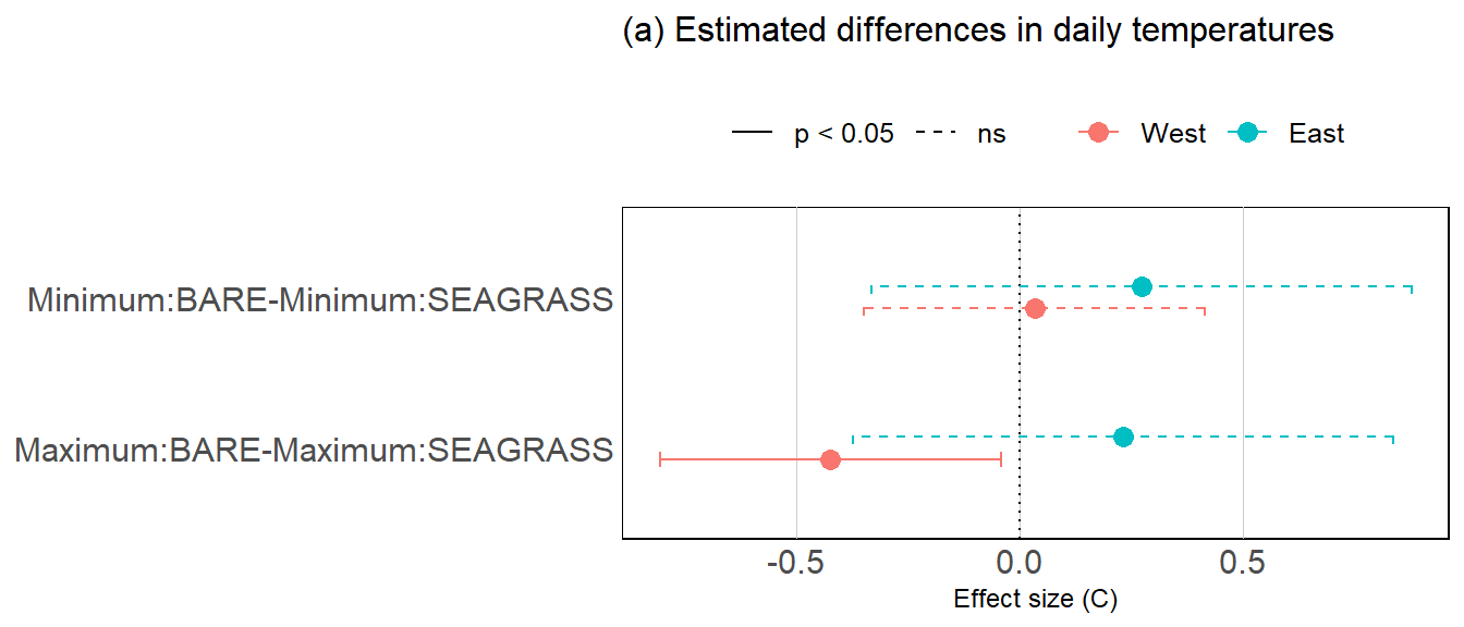
The same analysis is repeated but the daily temperature summaries are detrended by deployment date. This potentially reduces the effect of seasonal variation on the results.

Code

toplo <- dat %>% 
  mutate(
    date = date(datetime),
    stratum = factor(stratum, levels = c('SEAGRASS', 'BARE'))
  ) %>% 
  unite('grp', date, site) %>% 
  mutate(
    n = n(), 
    .by = c('grp')
  ) %>% 
  filter(n == 144) %>% 
  group_nest(deploy_date) %>% 
  mutate(
    data = purrr::map(data, function(x){
      
      mod <- lm(tempc ~ datetime, x)
      x$resid <- resid(mod)
      
      return(x)
      
    })
  ) %>% 
  unnest(data) %>% 
  summarise(
    minv = min(resid), 
    maxv = max(resid), 
    .by = c(grp, stratum, side)
  ) %>% 
  pivot_longer(names_to = 'met', values_to = 'tempc', minv:maxv) %>% 
  mutate(
    met = factor(met, levels = c('minv', 'maxv'), labels = c('Minimum', 'Maximum'))
  )


metcol <- c('dodgerblue', 'tomato1')
wd <- 1
p <- ggplot(toplo, aes(x = stratum, y = tempc, fill = met)) +
  geom_point(aes(color = met), position = position_jitterdodge(dodge.width = wd, jitter.width = 0.2), show.legend = F) +
  geom_boxplot(position = position_dodge(width = wd), outlier.colour = NA, alpha = 0.5) +
  scale_color_manual(values = metcol) + 
  scale_fill_manual(values = metcol) +
  facet_grid(~side) +
  theme_bw() +
  theme(
    strip.background = element_blank(), 
    panel.grid.minor = element_blank(), 
    legend.position = 'top', 
    strip.text = element_text(size = 12)
  ) + 
  labs(
    y = 'Detrended temp (C)', 
    x = NULL, 
    fill = 'Daily temperature'
  )
p

Code

sidemod <- toplo %>% 
  group_nest(side) %>% 
  mutate(
    mod = purrr::map(data, ~TukeyHSD(aov(tempc ~ met * stratum, data = .x)))
  )

toplo <- sidemod %>% 
  mutate(
    mod = purrr::map(mod, function(x){
      x$`met:stratum` %>% 
        data.frame %>% 
        mutate(
          comp = row.names(.)
        )
    })
  ) %>% 
  select(side, mod) %>% 
  unnest('mod') %>% 
  filter(comp %in% c("Minimum:BARE-Minimum:SEAGRASS", 
                     "Maximum:BARE-Maximum:SEAGRASS")
  ) %>% 
  mutate(
    pcol = ifelse(p.adj <= 0.05, 'p < 0.05', 'ns'), 
    pcol = factor(pcol, levels = c('p < 0.05', 'ns'))
  ) 

p <- ggplot(toplo, aes(y = comp, x = diff, linetype = pcol, col = side)) + 
  geom_vline(xintercept = 0, color = 'black', linetype = 'dotted') +
  geom_point(position = position_dodge(width = 0.3), size = 3) + 
  geom_errorbar(aes(xmin = lwr, xmax = upr), position = position_dodge(width = 0.3), width = 0.2) + 
  scale_linetype_manual(values = c('solid', 'dashed'), drop = F) +
  theme_ipsum(plot_margin = margin(5, 5, 5, 5)) + 
  theme(
    strip.placement = 'outside',
    panel.grid.minor = element_blank(),
    panel.grid.major.y = element_blank(),
    strip.background = element_blank(), 
    axis.title.y = element_blank(), 
    legend.title = element_blank(), 
    legend.position = 'top',
    axis.title.x = element_text(hjust = 0.5),
    strip.text.x = element_text(hjust = 0.5),
    strip.text = element_text(size = 9),
    panel.background = element_rect()
  ) +
  labs(
    x = 'Effect size (C)', 
    subtitle = '(a) Estimated differences in daily temperatures'
  )
p