library(tidyverse)
library(here)
library(patchwork)
# epc data by subsegment
load(file = here('data-clean/epcwq_clean.RData'))
epc <- epcwq3 |>
filter(param == 'Chla') |>
mutate(
date = ymd(date),
yr = year(date),
mo = month(date)
) |>
select(subsegment = subseg, mo, yr, obs = value, date) |>
summarise(
obs = mean(obs, na.rm = TRUE),
.by = c('subsegment', 'mo', 'yr', 'date')
)
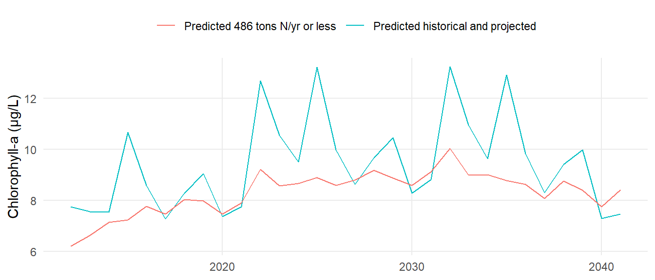
# casm data by subsegment
casm <- list(
"prd486" = read.csv(here("data-raw/casm486.csv")),
"prdhist" = read.csv(here("data-raw/casmhistproj.csv"))
) |>
enframe('run', 'data') |>
mutate(
data = map(data, function(x) x |>
pivot_longer(cols = -c(1:2), names_to = 'yr', values_to = 'prd') |>
rename(mo = Month) |>
mutate(
yr = gsub('X', '', yr) |> as.numeric(),
mo = factor(mo, levels = c('Jan', 'Feb', 'Mar', 'Apr', 'May', 'Jun', 'Jul', 'Aug', 'Sep', 'Oct', 'Nov', 'Dec'),
labels = c(1:12)) |> as.numeric(),
date = as.Date(paste0(yr, '-', mo, '-01'))
)
)
) |>
unnest('data') |>
pivot_wider(names_from = 'run', values_from = 'prd')
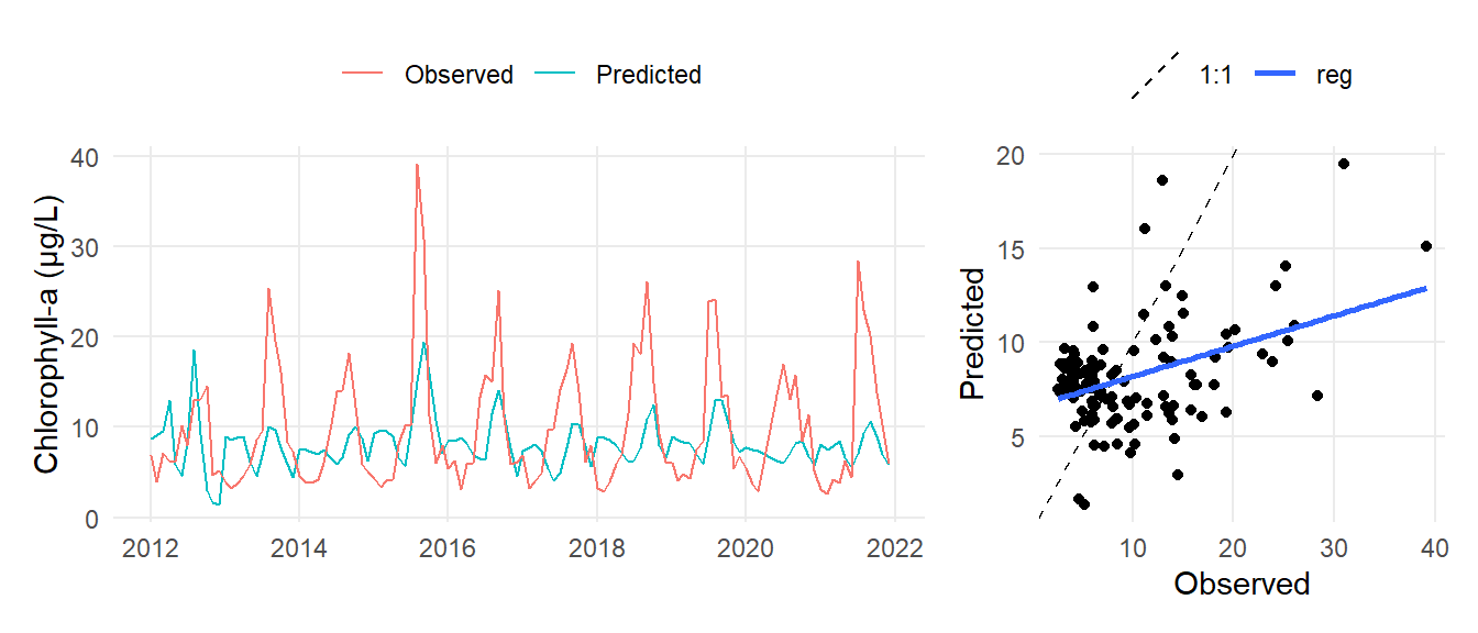
##
# combine epc and casm data
# monthly
mo <- casm |>
filter(yr <= 2021) |>
inner_join(epc, by = c('yr', 'mo', 'date', 'subsegment')) |>
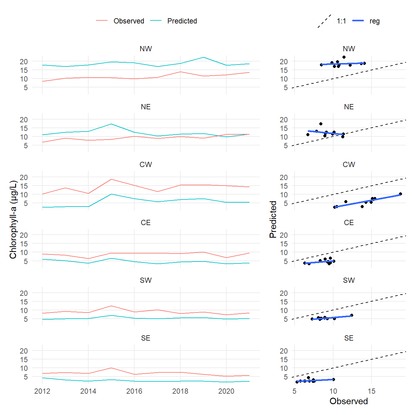
mutate(
subsegment = factor(subsegment, levels = c('NW', 'NE', 'CW', 'CE', 'SW', 'SE'))
)
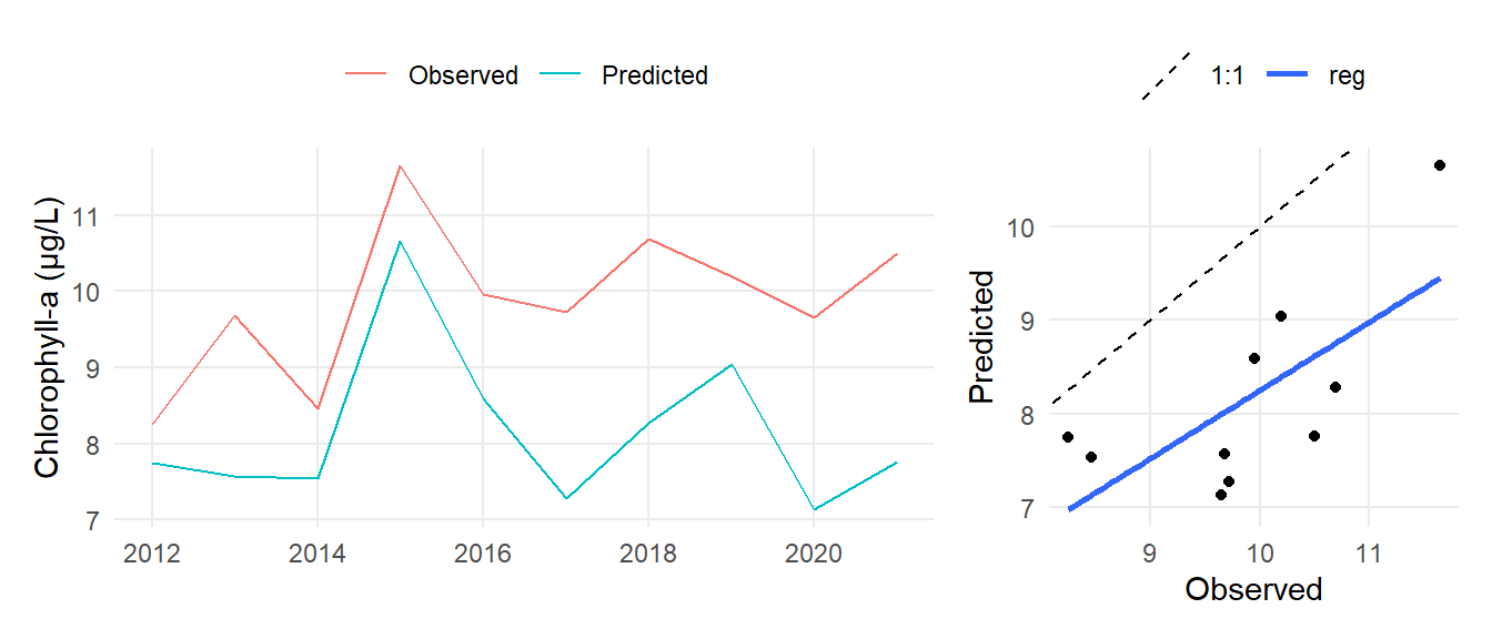
# annual
ann <- mo |>
summarise(
obs = mean(obs, na.rm = TRUE),
prd486 = mean(prd486, na.rm = TRUE),
prdhist = mean(prdhist, na.rm = TRUE),
.by = c('subsegment', 'yr')
)