Chlorophyll attainment by month, sub-segment

library(tidyverse)
library(tbeptools)
library(sjPlot)

load(file = here::here("data/otb_subseg_sites.RData"))
load(file = here::here("data/loads.RData"))

otbdat <- epcdata |> 
  filter(bay_segment == 'OTB') |> 
  mutate(
    epchc_station = as.character(epchc_station)
  ) |> 
  left_join(otb_subseg_sites, by = c('epchc_station' = 'site')) |> 
  filter(yr >= 2000 & yr <= 2021) |> 
  select(epchc_station, yr, mo, chla, tn, subsegment)

lddat <- loads |> 
  mutate(
    yr = year(date), 
    mo = month(date)
  ) |>
  filter(param == 'TN load') |> 
  select(yr, mo, load = value) |> 
  mutate(
    loadlag1 = lag(load, 1), 
    loadlag2 = lag(load, 2),
    loadlag3 = lag(load, 3),
    lagsum2 = loadlag1 + loadlag2,
    lagsum3 = loadlag1 + loadlag2 + loadlag3
  ) |> 
  filter(yr >= 2000 & yr <= 2021) 

ldplo <- lddat |> 
  summarise(
    load_av = mean(load, na.rm = T), 
    load_hi = t.test(load)$conf.int[2], 
    load_lo = t.test(load)$conf.int[1],
    .by = mo
  ) |> 
  mutate(
    load_pc = load_av / sum(load_av),
    load_486 = 486 * load_pc,
    lab = paste0(round(100 * load_pc, 1), '%')
  )

ldplo1 <- ldplo |> 
  select(mo, load_av, load_486) |> 
  pivot_longer(-mo) |>
  mutate(
    name = factor(name, levels = c('load_av', 'load_486'), 
                 labels = c('2000-2021 average', 'Absolute threshold')
    )
  )

ggplot(ldplo1, aes(x = mo)) + 
  geom_rect(data = ldplo1[1, ], aes(xmin = 5.5, xmax = 9.5, ymin = 0, ymax = Inf, fill = '2/3 annual average'), alpha = 0.2) +
  geom_line(data = lddat, aes(y = load, group = yr, color = 'Individual years'), alpha = 0.5) +
  geom_line(aes(y = value, color = name)) + 
  geom_point(aes(y = value, color = name)) +
  # geom_errorbar(data = ldplo, aes(ymin = load_lo, ymax = load_hi), width = 0)
  geom_text(data = ldplo, aes(label = lab, y = load_486), vjust = 1.5, color = '#00BFC4') +
  scale_color_manual(values = c('#F8766D', '#00BFC4', 'grey')) +
  scale_fill_manual(values = "grey") +
  labs(
    x = 'Month', 
    y = 'TN load (tons / month)', 
    color = NULL, 
    fill = NULL
  ) + 
  # scale_y_continuous(labels = scales::percent) +
  scale_x_continuous(breaks = 1:12) +
  theme_minimal() +
  theme(
    panel.grid.minor = element_blank(), 
    legend.position = 'top'
  )

NW sub-segment

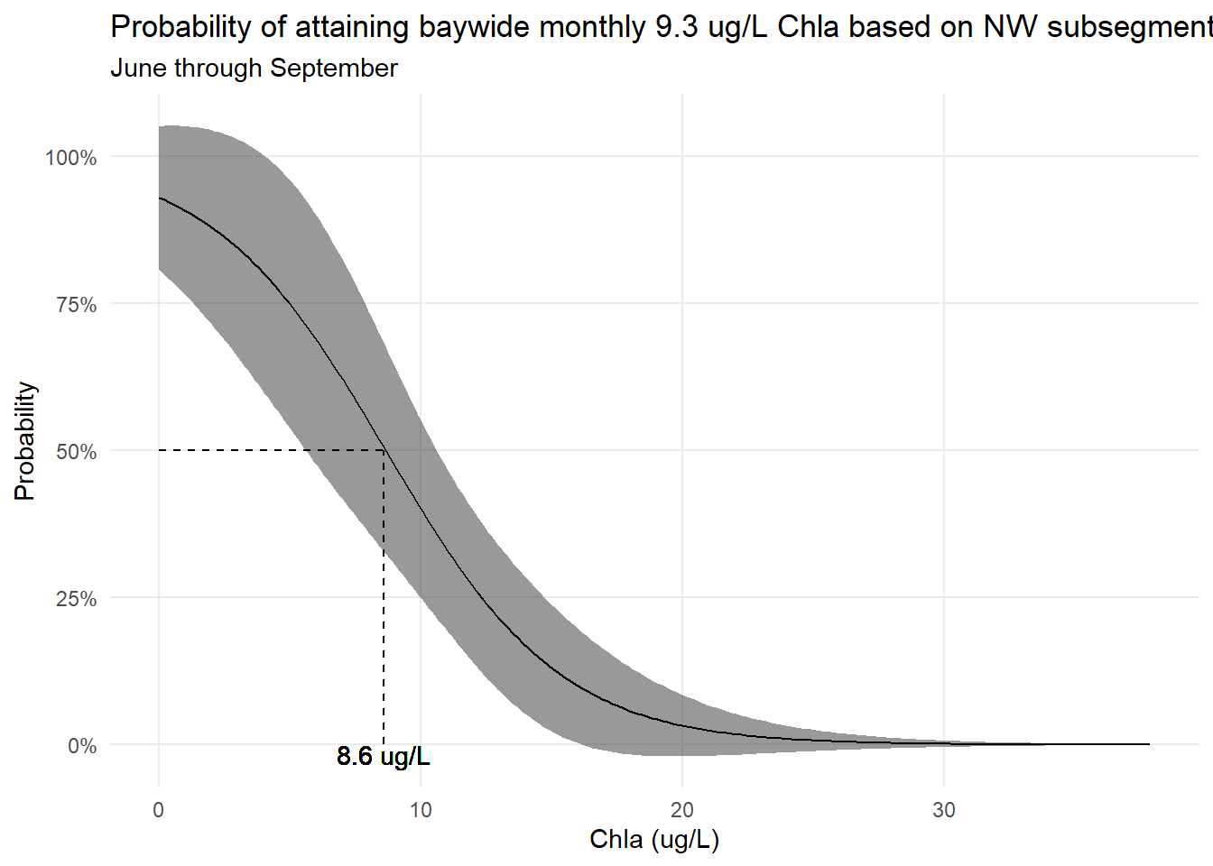
# monthly attainment whole bay segment, june through sep only
moattain <- otbdat |> 
  summarise(
    chla = mean(chla, na.rm = T), 
    .by = c('yr', 'mo')
  ) |>
  mutate(
    attain = chla < 9.3
  ) |> 
  select(-chla)

tomod <- otbdat |> 
  filter(mo %in% c(6:9)) |> 
  summarise(
    chla = mean(chla, na.rm = T), 
    .by = c(yr, mo, subsegment)
  ) |> 
  filter(subsegment == 'NW') |> 
  left_join(moattain, by = c('yr', 'mo')) 

mod <- glm(attain ~ chla, data = tomod, family = binomial)

prddat <- tibble(
    chla = seq(0, quantile(tomod$chla, 0.9), length.out = 200)
  )
prd <- tibble(
    ave = predict(mod, newdata = prddat, type = 'response'),
    lov = ave - predict(mod, newdata = prddat, type = 'response', se.fit = T)$se.fit * 1.96,
    hiv = ave + predict(mod, newdata = prddat, type = 'response', se.fit = T)$se.fit * 1.96
  ) |> 
  bind_cols(prddat)

# find chlorphyll value that is closes to lov 0.5
lns <- prd |> 
  mutate(
    diff = abs(0.5 - ave)
  ) |> 
  arrange(diff) |> 
  head(1)
lnslab <- paste0(round(lns$chla, 1), ' ug/L')

ggplot(prd, aes(x = chla, y = ave)) + 
  geom_ribbon(aes(ymin = lov, ymax = hiv), alpha = 0.5) + 
  geom_line() + 
  scale_y_continuous(labels = scales::percent) +
  geom_segment(x = lns$chla, xend = lns$chla, y = 0, yend = 0.5, linetype = 'dashed') +
  geom_segment(x = 0, xend = lns$chla, y = 0.5, yend = 0.5, linetype = 'dashed') +
  geom_text(x = lns$chla, y = 0, label = lnslab, vjust = 1) +
  labs(
    x = 'Chla (ug/L)', 
    y = 'Probability', 
    title = 'Probability of attaining baywide monthly 9.3 ug/L Chla based on NW subsegment concentrations',
    subtitle = 'June through September'
  ) + 
  theme_minimal() + 
  theme(
    panel.grid.minor = element_blank()
  )

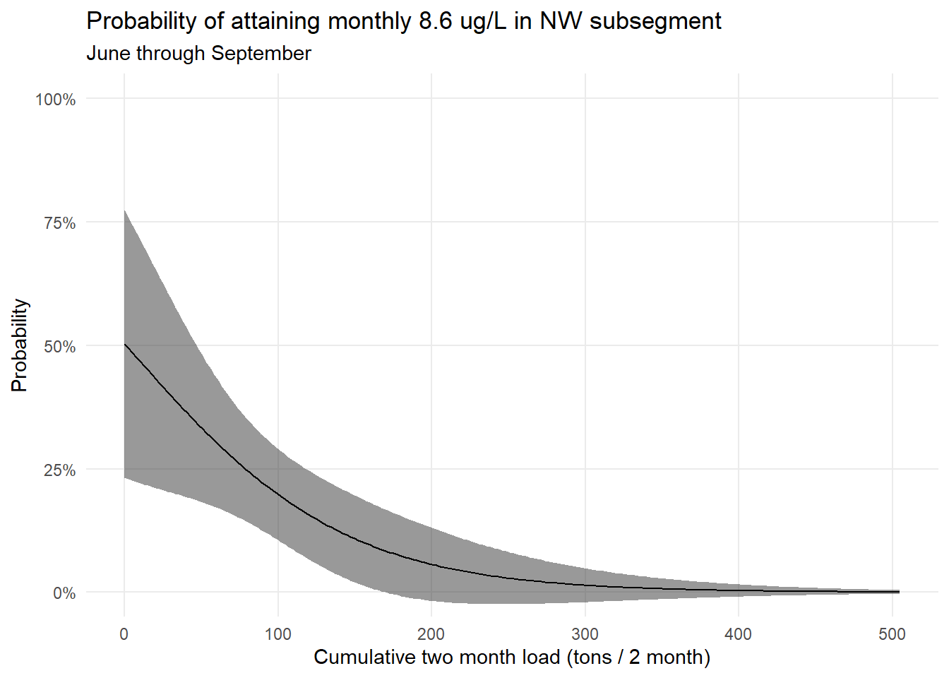
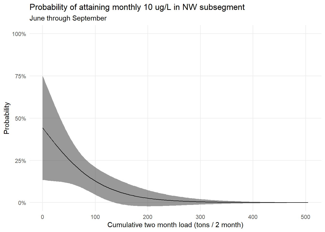
# probability of attaining monthly 50% chl value vs load
tomod2 <- tomod |> 
  mutate(
    attain = chla < lns$chla
  ) |> 
  left_join(lddat, by = c('yr', 'mo')) |> 
  mutate(
    mo = factor(mo),
    prdvar = lagsum2
  )

mod <- glm(attain ~ prdvar, data = tomod2, family = binomial)

prddat <- tibble(
    prdvar = seq(0, quantile(tomod2$prdvar, 1), length.out = 200)
  ) 
prd <- tibble(
    ave = predict(mod, newdata = prddat, type = 'response'),
    lov = ave - predict(mod, newdata = prddat, type = 'response', se.fit = T)$se.fit * 1.96,
    hiv = ave + predict(mod, newdata = prddat, type = 'response', se.fit = T)$se.fit * 1.96
  ) |> 
  bind_cols(prddat)

ggplot(prd, aes(x = prdvar, y = ave)) + 
  geom_ribbon(aes(ymin = lov, ymax = hiv), alpha = 0.5) + 
  geom_line() + 
  scale_y_continuous(labels = scales::percent) +
  coord_cartesian(ylim = c(0, 1)) + 
  labs(
    x = 'Cumulative two month load (tons / 2 month)', 
    y = 'Probability',
    title = paste('Probability of attaining monthly', lnslab, 'in NW subsegment'),
    subtitle = 'June through September'
  ) + 
  theme_minimal() + 
  theme(
    panel.grid.minor = element_blank()
  )

mod1 <- glm(attain ~ load, data = tomod2, family = binomial)
mod2 <- glm(attain ~ lagsum2, data = tomod2, family = binomial)
mod3 <- glm(attain ~ lagsum3, data = tomod2, family = binomial)
tab_model(mod1, mod2, mod3)

	attain			attain			attain
Predictors	Odds Ratios	CI	p	Odds Ratios	CI	p	Odds Ratios	CI	p
(Intercept)	0.31	0.10 – 0.94	0.035	1.01	0.35 – 3.08	0.982	1.15	0.36 – 3.94	0.822
load	1.00	0.99 – 1.01	0.613
lagsum2				0.99	0.97 – 1.00	0.012
lagsum3							0.99	0.98 – 1.00	0.013
Observations	88			88			88
R2 Tjur	0.003			0.111			0.107

CW sub-segment

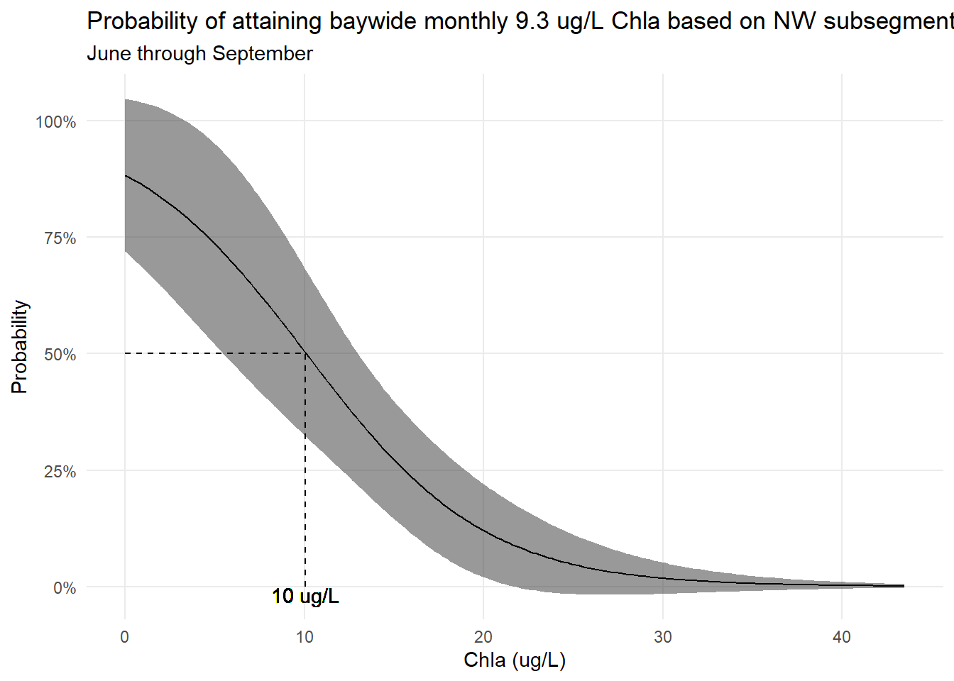
# monthly attainment whole bay segment, june through sep only
moattain <- otbdat |> 
  summarise(
    chla = mean(chla, na.rm = T), 
    .by = c('yr', 'mo')
  ) |>
  mutate(
    attain = chla < 9.3
  ) |> 
  select(-chla)

tomod <- otbdat |> 
  filter(mo %in% c(6:9)) |> 
  summarise(
    chla = mean(chla, na.rm = T), 
    .by = c(yr, mo, subsegment)
  ) |> 
  filter(subsegment == 'CW') |> 
  left_join(moattain, by = c('yr', 'mo')) 

mod <- glm(attain ~ chla, data = tomod, family = binomial)

prddat <- tibble(
    chla = seq(0, quantile(tomod$chla, 0.9), length.out = 200)
  )
prd <- tibble(
    ave = predict(mod, newdata = prddat, type = 'response'),
    lov = ave - predict(mod, newdata = prddat, type = 'response', se.fit = T)$se.fit * 1.96,
    hiv = ave + predict(mod, newdata = prddat, type = 'response', se.fit = T)$se.fit * 1.96
  ) |> 
  bind_cols(prddat)

# find chlorphyll value that is closes to lov 0.5
lns <- prd |> 
  mutate(
    diff = abs(0.5 - ave)
  ) |> 
  arrange(diff) |> 
  head(1)
lnslab <- paste0(round(lns$chla, 1), ' ug/L')

ggplot(prd, aes(x = chla, y = ave)) + 
  geom_ribbon(aes(ymin = lov, ymax = hiv), alpha = 0.5) + 
  geom_line() + 
  scale_y_continuous(labels = scales::percent) +
  geom_segment(x = lns$chla, xend = lns$chla, y = 0, yend = 0.5, linetype = 'dashed') +
  geom_segment(x = 0, xend = lns$chla, y = 0.5, yend = 0.5, linetype = 'dashed') +
  geom_text(x = lns$chla, y = 0, label = lnslab, vjust = 1) +
  labs(
    x = 'Chla (ug/L)', 
    y = 'Probability', 
    title = 'Probability of attaining baywide monthly 9.3 ug/L Chla based on NW subsegment concentrations',
    subtitle = 'June through September'
  ) + 
  theme_minimal() + 
  theme(
    panel.grid.minor = element_blank()
  )

# probability of attaining monthly 50% chl value vs load
tomod2 <- tomod |> 
  mutate(
    attain = chla < lns$chla
  ) |> 
  left_join(lddat, by = c('yr', 'mo')) |> 
  mutate(
    mo = factor(mo),
    prdvar = lagsum2
  )

mod <- glm(attain ~ prdvar, data = tomod2, family = binomial)

prddat <- tibble(
    prdvar = seq(0, quantile(tomod2$prdvar, 1), length.out = 200)
  ) 
prd <- tibble(
    ave = predict(mod, newdata = prddat, type = 'response'),
    lov = ave - predict(mod, newdata = prddat, type = 'response', se.fit = T)$se.fit * 1.96,
    hiv = ave + predict(mod, newdata = prddat, type = 'response', se.fit = T)$se.fit * 1.96
  ) |> 
  bind_cols(prddat)

ggplot(prd, aes(x = prdvar, y = ave)) + 
  geom_ribbon(aes(ymin = lov, ymax = hiv), alpha = 0.5) + 
  geom_line() + 
  scale_y_continuous(labels = scales::percent) +
  coord_cartesian(ylim = c(0, 1)) + 
  labs(
    x = 'Cumulative two month load (tons / 2 month)', 
    y = 'Probability',
    title = paste('Probability of attaining monthly', lnslab, 'in NW subsegment'),
    subtitle = 'June through September'
  ) + 
  theme_minimal() + 
  theme(
    panel.grid.minor = element_blank()
  )

mod1 <- glm(attain ~ load, data = tomod2, family = binomial)
mod2 <- glm(attain ~ lagsum2, data = tomod2, family = binomial)
mod3 <- glm(attain ~ lagsum3, data = tomod2, family = binomial)
tab_model(mod1, mod2, mod3)

	attain			attain			attain
Predictors	Odds Ratios	CI	p	Odds Ratios	CI	p	Odds Ratios	CI	p
(Intercept)	0.22	0.06 – 0.82	0.021	0.80	0.23 – 2.85	0.720	1.18	0.29 – 5.28	0.818
load	1.00	0.98 – 1.01	0.566
lagsum2				0.98	0.97 – 1.00	0.019
lagsum3							0.98	0.97 – 0.99	0.013
Observations	88			88			88
R2 Tjur	0.004			0.107			0.125