Load projections

Code

library(tidyverse)

load(file = here::here('data-raw/mosdat.RData'))
load(file = here::here('data-raw/mohydat.RData'))
load(file = here::here('data-raw/tnanndat.RData'))

lddat <- mosdat |> 
  filter(bay_segment == 'Old Tampa Bay') |> 
  filter(year >= 2000 & year <= 2021) |> 
  summarise(
    tn_load = sum(tn_load),
    tp_load = sum(tp_load),
    tss_load = sum(tss_load),
    .by = 'year'
  )

npslddat <- mosdat |> 
  filter(bay_segment == 'Old Tampa Bay') |>
  filter(source == 'NPS') |> 
  filter(year >= 2000 & year <= 2021) |> 
  summarise(
    tn_load = sum(tn_load), 
    .by = 'year'
  )

hymodat <- mohydat |> 
  filter(bay_segment == 'Old Tampa Bay') |> 
  filter(year >= 2000 & year <= 2021) |> 
  select(year, month, hy_load = hy_load_106_m3_mo)
hydat <- hymodat |> 
  summarise(
    hy_load = sum(hy_load),
    .by = 'year'
  )
casmdat <- read.fwf(
  here::here('data-raw/OTB-DailyLoads2000-2021.dat'),
  widths = c(5, 4, 4, 5, 5, 12, 12, 12),
  header = F,
  skip = 1,
  stringsAsFactors = FALSE,
  col.names = c("Year", "Yr", "Mo", "Day", "DOY", "TN tons/d", "TP tons/d", "TSS tons/d")
)

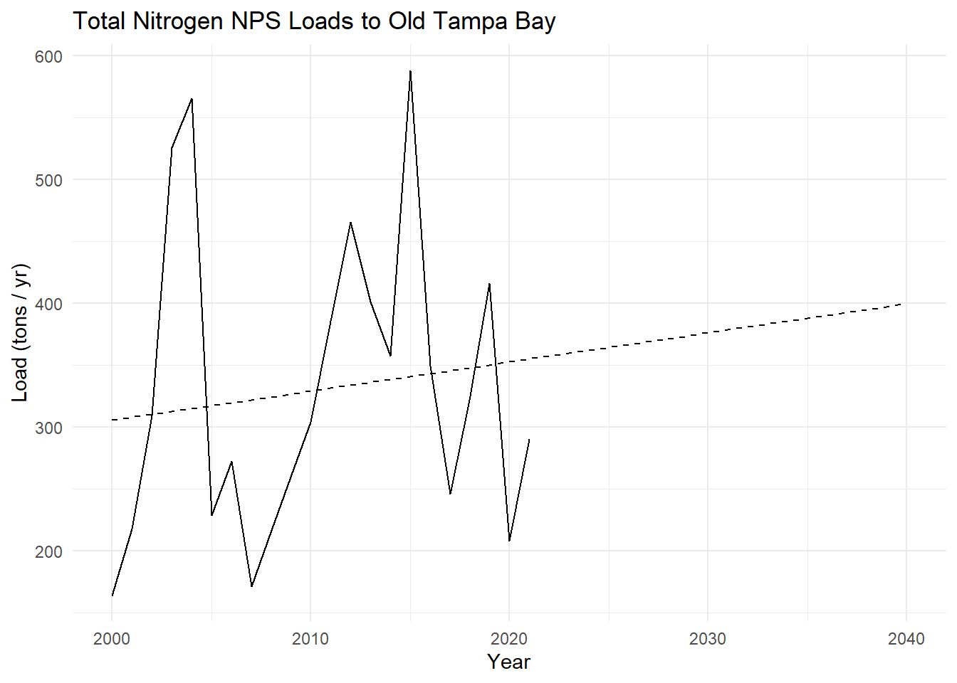
This document shows a projection of estimated load change to 2040 based on annual loading estimates from 2000 to 2021.

Total Nitrogen

Code

# regression model of tn_load by year
tnmod <- lm(tn_load ~ year, data = npslddat)

# get predictions for years 1985:2040
preds <- data.frame(year = 2000:2040)
preds <- preds |> 
  mutate(
    tn_load = predict(tnmod, preds)
  )

# plot tn_load as line plot by year
# add regression predictions
p <- ggplot(npslddat, aes(x = year, y = tn_load)) +
  geom_line() +
  geom_line(data = preds, linetype = 'dashed') +
  labs(title = 'Total Nitrogen NPS Loads to Old Tampa Bay',
       x = 'Year',
       y = 'Load (tons / yr)'
  ) +
  theme_minimal()
p

Code

# estimate means from 2000 to 2021 and 2040
means <- preds |> 
  summarise(
    mean_load_2000_2021 = mean(tn_load[year >= 2000 & year <= 2021]),
    mean_load_2040 = mean(tn_load[year == 2040])
  )

# take percent change from 2000 to 2021 to 2040
means <- means |> 
  mutate(
    percent_change = (mean_load_2040 - mean_load_2000_2021) / mean_load_2000_2021 * 100
  )
means

  mean_load_2000_2021 mean_load_2040 percent_change
1            330.2616       399.7735       21.04753

NPS is only a portion of the TN load in a given year. The percentages each year are:

Code

npsper <- tnanndat |> 
  filter(bay_segment == 'Old Tampa Bay') |> 
  filter(year >= 2000 & year <= 2021) |> 
  pivot_wider(names_from = source, values_from = tn_load) |> 
  mutate(
    nps_percent = NPS / (AD + DPS + GWS + IPS + NPS) * 100, 
    tn_change = NULL
  ) |> 
  select(year, nps_percent)
npsper

# A tibble: 22 × 2
    year nps_percent
   <dbl>       <dbl>
 1  2000        41.3
 2  2001        49.0
 3  2002        50.2
 4  2003        59.0
 5  2004        66.0
 6  2005        48.6
 7  2006        52.7
 8  2007        43.9
 9  2008        50.4
10  2009        51.3
# ℹ 12 more rows

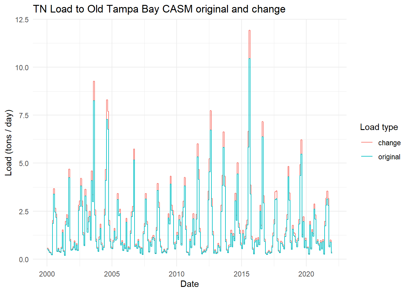
The NPS percent each year is joined to the CASM file and the proportion of the TN load that is NPS is extracted and changed by the estimated percent change from above.

Code

npschg <- means |> 
  pull(percent_change)
casmdat <- casmdat |> 
  left_join(npsper, by = c('Year' = 'year')) |> 
  mutate(
    nps_tn = TN.tons.d * nps_percent / 100,
    tn_change = TN.tons.d * nps_percent / 100 * npschg / 100, 
    TN.tons.d.chg = TN.tons.d + tn_change
  )
head(casmdat)

  Year Yr Mo Day DOY TN.tons.d TP.tons.d TSS.tons.d nps_percent    nps_tn
1 2000  1  1   1   1     0.519    0.2894      3.975    41.30117 0.2143531
2 2000  1  1   2   2     0.519    0.2894      3.975    41.30117 0.2143531
3 2000  1  1   3   3     0.519    0.2894      3.975    41.30117 0.2143531
4 2000  1  1   4   4     0.519    0.2894      3.975    41.30117 0.2143531
5 2000  1  1   5   5     0.519    0.2894      3.975    41.30117 0.2143531
6 2000  1  1   6   6     0.519    0.2894      3.975    41.30117 0.2143531
   tn_change TN.tons.d.chg
1 0.04511602      0.564116
2 0.04511602      0.564116
3 0.04511602      0.564116
4 0.04511602      0.564116
5 0.04511602      0.564116
6 0.04511602      0.564116

For comparison, the original TN tons/d can be plotted relative to the change.

Code

toplo <- casmdat |> 
  mutate(
    date = as.Date(paste(Year, Mo, Day, sep = '-'))
  ) |> 
  select(date, original = TN.tons.d, change = TN.tons.d.chg) |> 
  pivot_longer(cols = c(original, change), names_to = 'var', values_to = 'load')

p <- ggplot(toplo, aes(x = date, y = load, color = var)) +
  geom_line() +
  theme_minimal() + 
  labs(title = 'TN Load to Old Tampa Bay CASM original and change',
       x = 'Date',
       y = 'Load (tons / day)',
       color = 'Load type')
p

Verify the percent change is correct.

Code

casmdat |> 
  mutate(
    npschg = tn_change / (TN.tons.d * (nps_percent / 100))
  ) |> 
  select(Year, npschg) |> 
  pull(npschg) |> 
  unique() |> 
  mean()

[1] 0.2104753

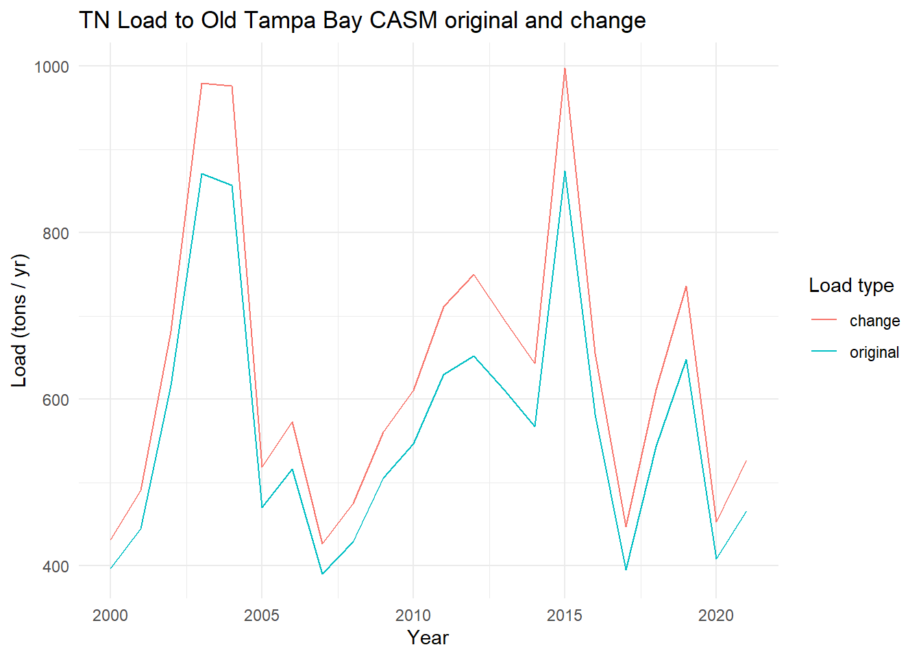
View the total annual TN from before and with the change.

Code

toplo <- casmdat |> 
  summarise(
    original = sum(TN.tons.d),
    change = sum(TN.tons.d.chg), 
    .by = Year
  ) |> 
  pivot_longer(cols = c(original, change), names_to = 'var', values_to = 'load')

p <- ggplot(toplo, aes(x = Year, y = load, color = var)) +
  geom_line() +
  theme_minimal() + 
  labs(title = 'TN Load to Old Tampa Bay CASM original and change',
       x = 'Year',
       y = 'Load (tons / yr)',
       color = 'Load type')
p

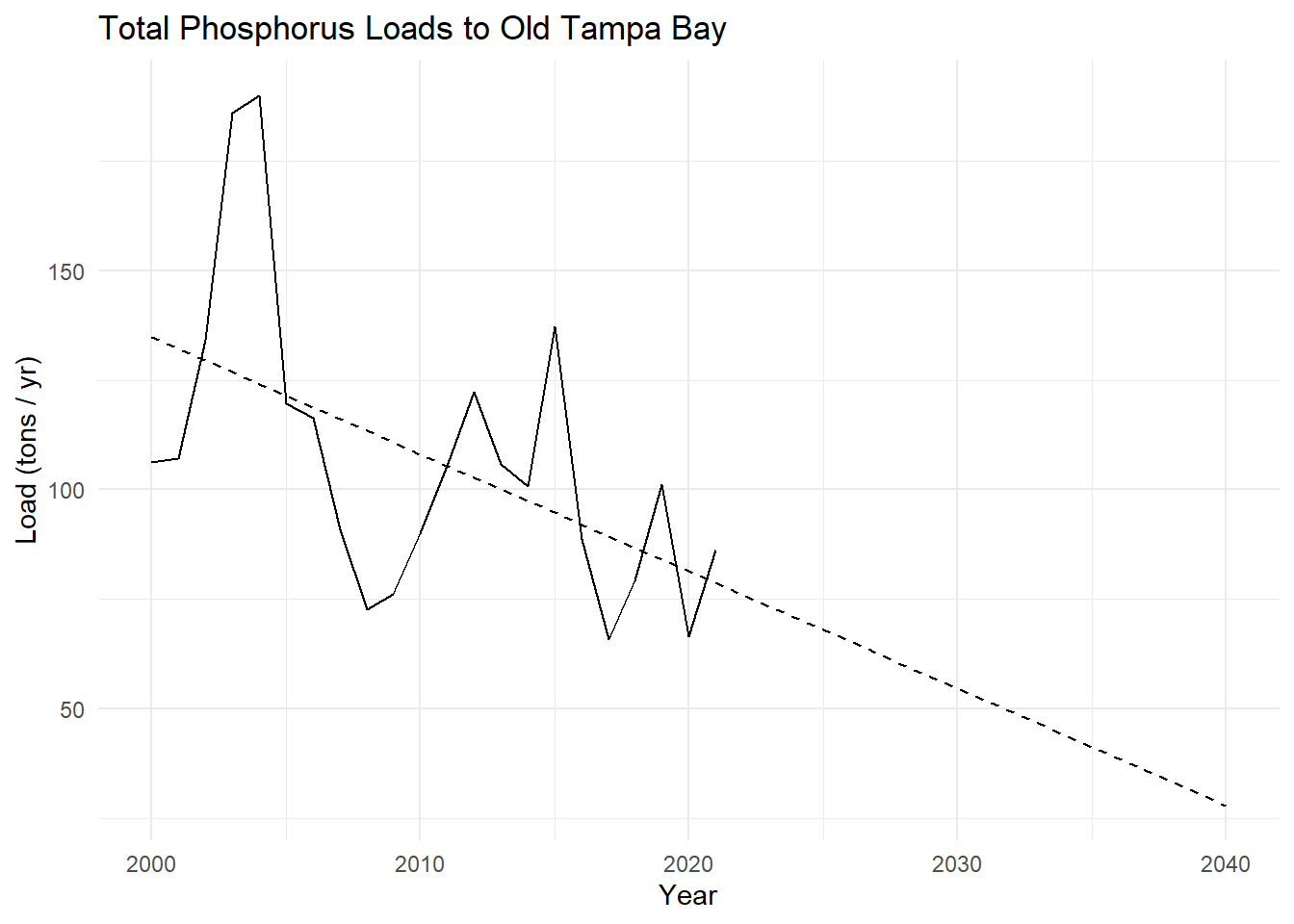
Total Phosphorus

Do the same for total phosphorus.

Code

# regression model of tn_load by year
tpmod <- lm(tp_load ~ year, data = lddat)

# get predictions for years 1985:2040
preds <- data.frame(year = 2000:2040)
preds <- preds |> 
  mutate(
    tp_load = predict(tpmod, preds)
  )

# plot tn_load as line plot by year
# add regression predictions
p <- ggplot(lddat, aes(x = year, y = tp_load)) +
  geom_line() +
  geom_line(data = preds, linetype = 'dashed') +
  labs(title = 'Total Phosphorus Loads to Old Tampa Bay',
       x = 'Year',
       y = 'Load (tons / yr)',
       color = 'Load type') +
  theme_minimal()
p

Code

# estimate means from 2000 to 2021 and 2040
means <- preds |> 
  summarise(
    mean_load_2000_2021 = mean(tp_load[year >= 2000 & year <= 2021]),
    mean_load_2040 = mean(tp_load[year == 2040])
  )

# take percent change from 2000 to 2021 to 2040
means <- means |> 
  mutate(
    percent_change = (mean_load_2040 - mean_load_2000_2021) / mean_load_2000_2021 * 100
  )
means

  mean_load_2000_2021 mean_load_2040 percent_change
1            106.7255       27.90491      -73.85357

The TP load is changed by the estimated percent change from above.

Code

tpchg <- means |> 
  pull(percent_change)
casmdat <- casmdat |> 
  select(-nps_percent, -nps_tn, -tn_change) |>
  mutate(
    TP.tons.d.chg = TP.tons.d + TP.tons.d * (tpchg / 100)
  )
head(casmdat)

  Year Yr Mo Day DOY TN.tons.d TP.tons.d TSS.tons.d TN.tons.d.chg TP.tons.d.chg
1 2000  1  1   1   1     0.519    0.2894      3.975      0.564116    0.07566777
2 2000  1  1   2   2     0.519    0.2894      3.975      0.564116    0.07566777
3 2000  1  1   3   3     0.519    0.2894      3.975      0.564116    0.07566777
4 2000  1  1   4   4     0.519    0.2894      3.975      0.564116    0.07566777
5 2000  1  1   5   5     0.519    0.2894      3.975      0.564116    0.07566777
6 2000  1  1   6   6     0.519    0.2894      3.975      0.564116    0.07566777

For comparison, the original TP tons/d can be plotted relative to the change.

Code

toplo <- casmdat |> 
  mutate(
    date = as.Date(paste(Year, Mo, Day, sep = '-'))
  ) |> 
  select(date, original = TP.tons.d, change = TP.tons.d.chg) |> 
  pivot_longer(cols = c(original, change), names_to = 'var', values_to = 'load')

p <- ggplot(toplo, aes(x = date, y = load, color = var)) +
  geom_line() +
  theme_minimal() + 
  labs(title = 'TP Load to Old Tampa Bay CASM original and change',
       x = 'Date',
       y = 'Load (tons / day)',
       color = 'Load type')
p

Verify the percent change is correct.

Code

casmdat |> 
  mutate(
    tpchg = (TP.tons.d.chg - TP.tons.d) / TP.tons.d
  ) |> 
  select(Year, tpchg) |> 
  pull(tpchg) |> 
  unique() |> 
  mean()

[1] -0.7385357

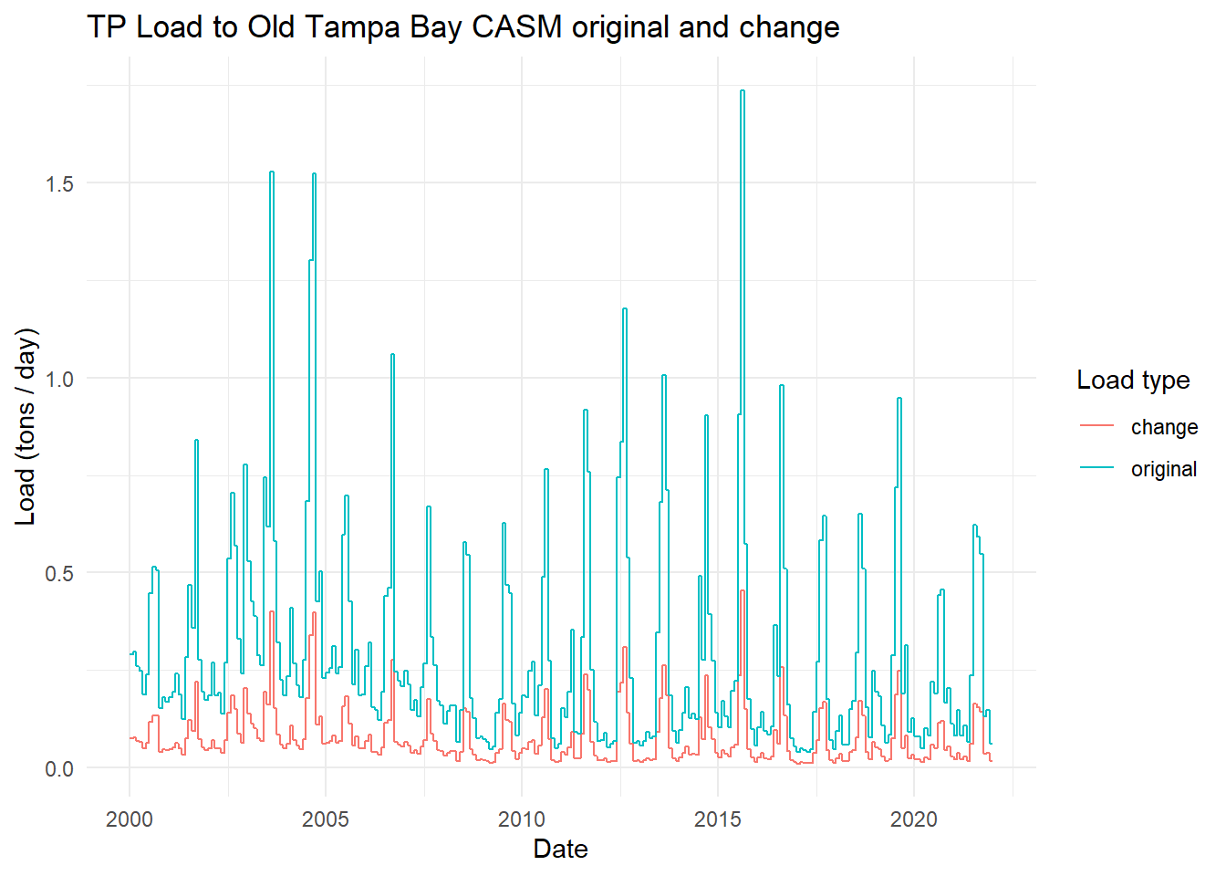
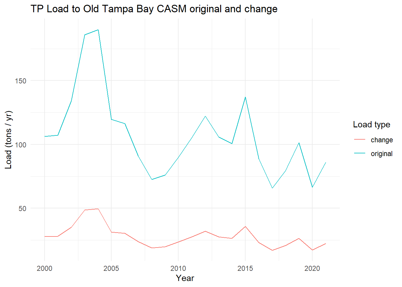
View the total annual TP from before and with the change.

Code

toplo <- casmdat |> 
  summarise(
    original = sum(TP.tons.d),
    change = sum(TP.tons.d.chg), 
    .by = Year
  ) |> 
  pivot_longer(cols = c(original, change), names_to = 'var', values_to = 'load')

p <- ggplot(toplo, aes(x = Year, y = load, color = var)) +
  geom_line() +
  theme_minimal() + 
  labs(title = 'TP Load to Old Tampa Bay CASM original and change',
       x = 'Year',
       y = 'Load (tons / yr)',
       color = 'Load type')
p

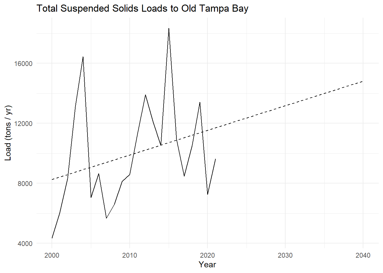
Total Suspended Solids

Do the same for total suspended solids.

Code

# regression model of tn_load by year
tssmod <- lm(tss_load ~ year, data = lddat)

# get predictions for years 1985:2040
preds <- data.frame(year = 2000:2040)
preds <- preds |> 
  mutate(
    tss_load = predict(tssmod, preds)
  )

# plot tn_load as line plot by year
# add regression predictions
p <- ggplot(lddat, aes(x = year, y = tss_load)) +
  geom_line() +
  geom_line(data = preds, linetype = 'dashed') +
  labs(title = 'Total Suspended Solids Loads to Old Tampa Bay',
       x = 'Year',
       y = 'Load (tons / yr)',
       color = 'Load type') +
  theme_minimal()
p

Code

# estimate means from 2000 to 2021 and 2040
means <- preds |> 
  summarise(
    mean_load_2000_2021 = mean(tss_load[year >= 2000 & year <= 2021]),
    mean_load_2040 = mean(tss_load[year == 2040])
  )

# take percent change from 2000 to 2021 to 2040
means <- means |> 
  mutate(
    percent_change = (mean_load_2040 - mean_load_2000_2021) / mean_load_2000_2021 * 100
  )
means

  mean_load_2000_2021 mean_load_2040 percent_change
1             9972.58       14811.54       48.52262

The TSS load is changed by the estimated percent change from above.

Code

tsschg <- means |> 
  pull(percent_change)
casmdat <- casmdat |> 
  mutate(
    TSS.tons.d.chg = TSS.tons.d + TSS.tons.d * (tsschg / 100)
  )
head(casmdat)

  Year Yr Mo Day DOY TN.tons.d TP.tons.d TSS.tons.d TN.tons.d.chg TP.tons.d.chg
1 2000  1  1   1   1     0.519    0.2894      3.975      0.564116    0.07566777
2 2000  1  1   2   2     0.519    0.2894      3.975      0.564116    0.07566777
3 2000  1  1   3   3     0.519    0.2894      3.975      0.564116    0.07566777
4 2000  1  1   4   4     0.519    0.2894      3.975      0.564116    0.07566777
5 2000  1  1   5   5     0.519    0.2894      3.975      0.564116    0.07566777
6 2000  1  1   6   6     0.519    0.2894      3.975      0.564116    0.07566777
  TSS.tons.d.chg
1       5.903774
2       5.903774
3       5.903774
4       5.903774
5       5.903774
6       5.903774

For comparison, the original TSS tons/d can be plotted relative to the change.

Code

toplo <- casmdat |> 
  mutate(
    date = as.Date(paste(Year, Mo, Day, sep = '-'))
  ) |> 
  select(date, original = TSS.tons.d, change = TSS.tons.d.chg) |> 
  pivot_longer(cols = c(original, change), names_to = 'var', values_to = 'load')

p <- ggplot(toplo, aes(x = date, y = load, color = var)) +
  geom_line() +
  theme_minimal() + 
  labs(title = 'TSS Load to Old Tampa Bay CASM original and change',
       x = 'Date',
       y = 'Load (tons / day)',
       color = 'Load type')
p

Verify the percent change is correct.

Code

casmdat |> 
  mutate(
    tsschg = (TSS.tons.d.chg - TSS.tons.d) / TSS.tons.d
  ) |> 
  select(Year, tsschg) |> 
  pull(tsschg) |> 
  unique() |> 
  mean()

[1] 0.4852262

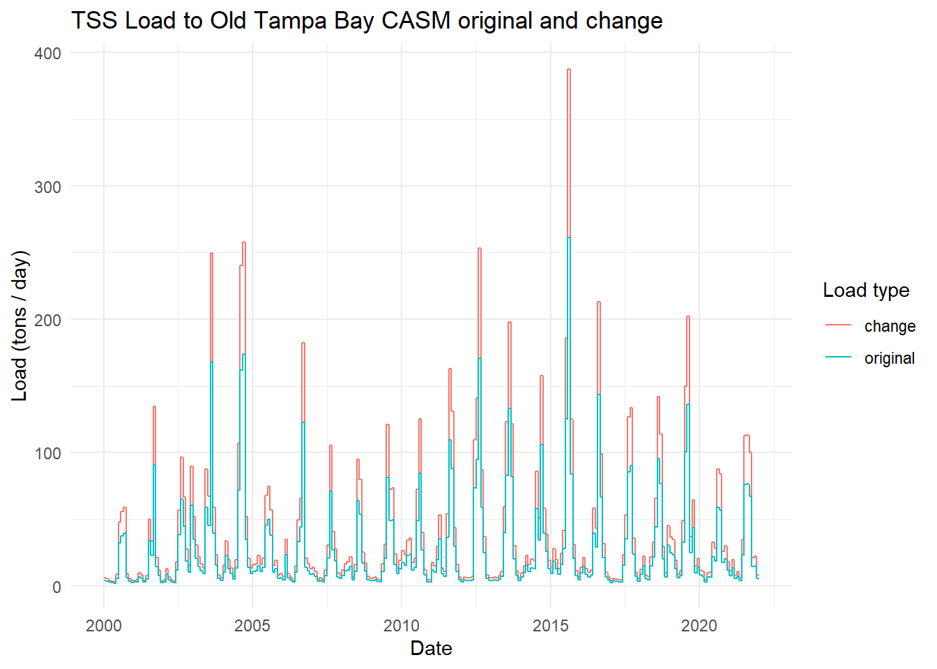
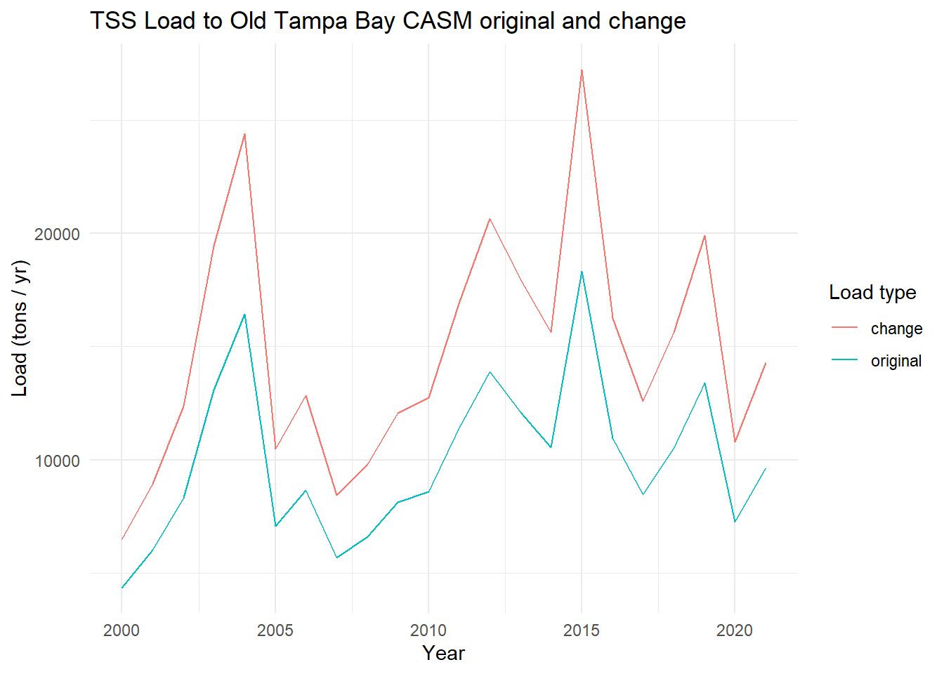
View the total annual TSS from before and with the change.

Code

toplo <- casmdat |> 
  summarise(
    original = sum(TSS.tons.d),
    change = sum(TSS.tons.d.chg), 
    .by = Year
  ) |> 
  pivot_longer(cols = c(original, change), names_to = 'var', values_to = 'load')

p <- ggplot(toplo, aes(x = Year, y = load, color = var)) +
  geom_line() +
  theme_minimal() + 
  labs(title = 'TSS Load to Old Tampa Bay CASM original and change',
       x = 'Year',
       y = 'Load (tons / yr)',
       color = 'Load type')
p

Save CASM file

Write the updated CASM file to disk using the same column widths as the input file.

Code

write_fixed_width <- function(df, file) {
  
  # Open file connection
  con <- file(file, "w")
  
  # Write header with exact spacing
  writeLines("Year  Yr  Mo  Day  DOY   TN tons/d   TP tons/d   TSS tons/d", con)
  
  # Write data rows
  for(i in 1:nrow(df)) {
    # Format each column with precise spacing and scientific notation
    line <- sprintf("%5d %3d %3d %4d %4d  %10.4E  %10.4E  %10.4E",
                    df$Year[i], df$Yr[i], df$Mo[i], df$Day[i], df$DOY[i],
                    df$`TN tons/d`[i], df$`TP tons/d`[i], df$`TSS tons/d`[i])
    writeLines(line, con)
  }
  
  # Close file connection
  close(con)
  
}

casmdat <- casmdat |> 
  select(Year, Yr, Mo, Day, DOY, `TN tons/d` = TN.tons.d.chg, `TP tons/d` = TP.tons.d.chg, `TSS tons/d` = TSS.tons.d.chg)
write_fixed_width(casmdat, here::here('data-raw/OTB-DailyLoads2000-2021-chg.dat'))

Hydrology

Code

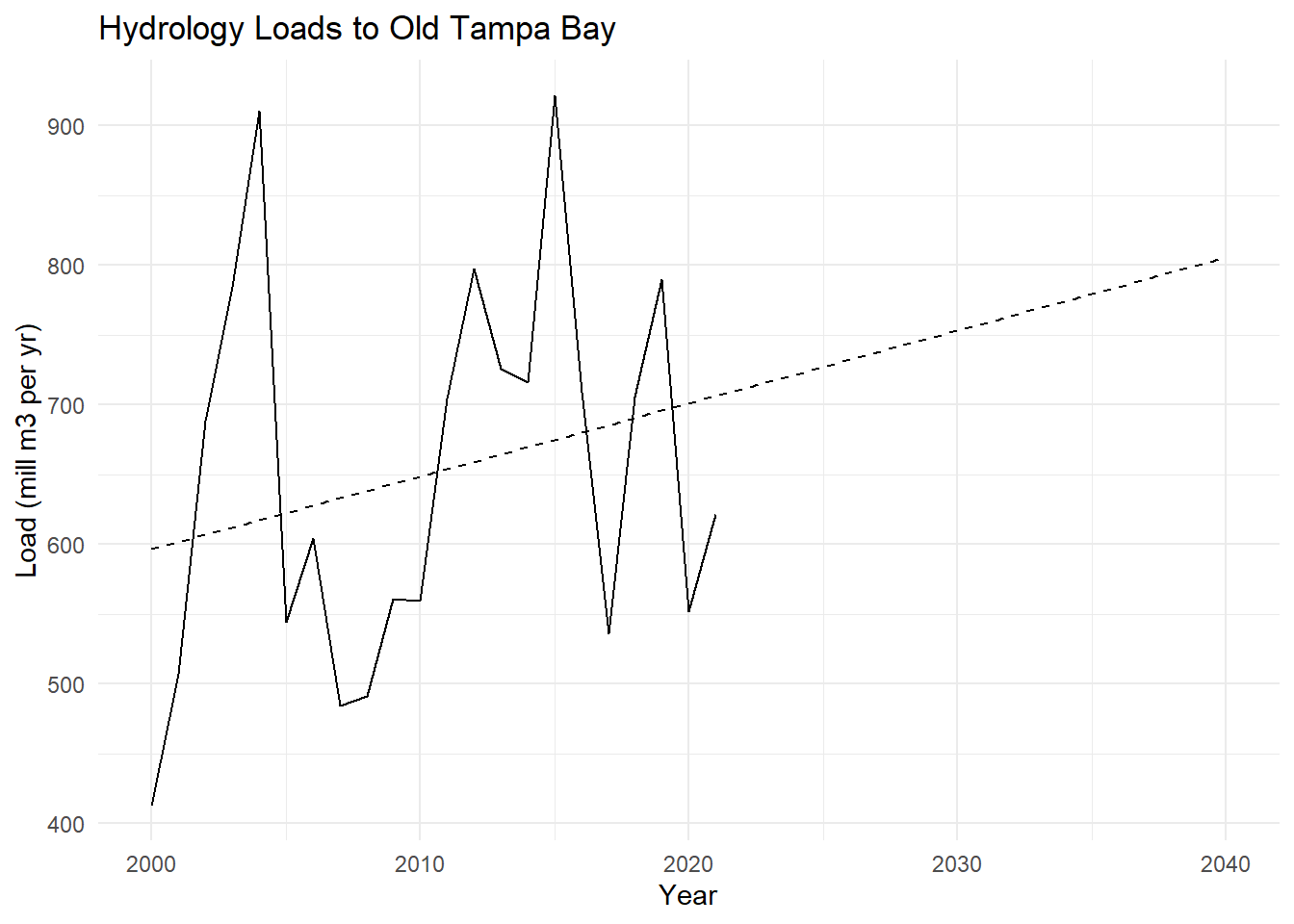
# regression model of hy_load by year
hymod <- lm(hy_load ~ year, data = hydat)

# get predictions for years 1985:2040
preds <- data.frame(year = 2000:2040)
preds <- preds |> 
  mutate(
    hy_load = predict(hymod, preds)
  )

# plot hy_load as line plot by year
# add regression predictions
p <- ggplot(hydat, aes(x = year, y = hy_load)) +
  geom_line() +
  geom_line(data = preds, linetype = 'dashed') +
  labs(title = 'Hydrology Loads to Old Tampa Bay',
       x = 'Year',
       y = 'Load (mill m3 per yr)') +
  theme_minimal()
p

Code

# estimate means from 2000 to 2021 and 2040
means <- preds |> 
  summarise(
    mean_load_2000_2021 = mean(hy_load[year >= 2000 & year <= 2021]),
    mean_load_2040 = mean(hy_load[year == 2040])
  )

# take percent change from 2000 to 2021 to 2040
means <- means |> 
  mutate(
    percent_change = (mean_load_2040 - mean_load_2000_2021) / mean_load_2000_2021 * 100
  )
means

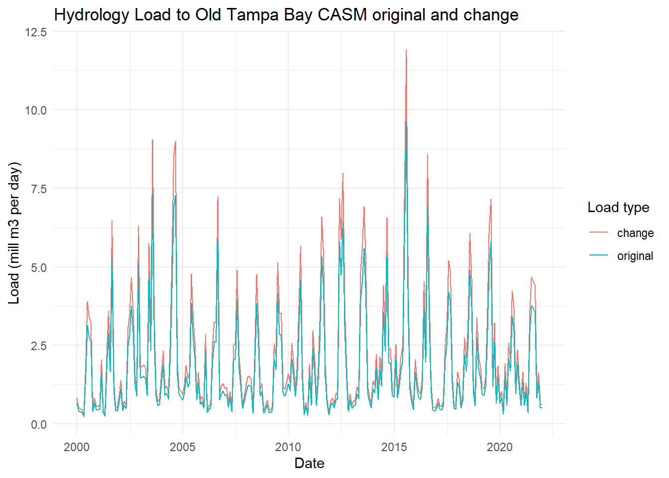
  mean_load_2000_2021 mean_load_2040 percent_change
1            651.2472       805.5106       23.68737

Because hydrology is not in the CASM file, we create a daily time series using linear interpolation of the monthly data. This is done to apply the estimated percent change from above.

Code

# create daily time series
hydlydat <- hymodat |> 
  mutate(
    date = lubridate::make_date(year, month, 1),
    hy_load = hy_load / days_in_month(date)
  ) |> 
  select(date, hy_load) |> 
  complete(date = seq.Date(min(date), lubridate::ceiling_date(max(date), 'month') - days(1), by = 'day')) |> 
  mutate(
    hy_load = approx(x = date, y = hy_load, xout = date)$y
  ) |> 
  fill(hy_load, .direction = 'down')

# apply change
hychg <- means |> 
  pull(percent_change)
hydlydat <- hydlydat |> 
  mutate(
    hy_load_chg = hy_load + hy_load * (hychg / 100)
  )
head(hydlydat)

# A tibble: 6 × 3
  date       hy_load hy_load_chg
  <date>       <dbl>       <dbl>
1 2000-01-01   0.673       0.833
2 2000-01-02   0.665       0.822
3 2000-01-03   0.656       0.812
4 2000-01-04   0.648       0.801
5 2000-01-05   0.639       0.791
6 2000-01-06   0.631       0.780

For comparison, the original linearly interpolated hydrology load can be plotted relative to the change.

Code

toplo <- hydlydat |> 
  select(date, original = hy_load, change = hy_load_chg) |> 
  pivot_longer(cols = c(original, change), names_to = 'var', values_to = 'load')

p <- ggplot(toplo, aes(x = date, y = load, color = var)) +
  geom_line() +
  theme_minimal() + 
  labs(title = 'Hydrology Load to Old Tampa Bay CASM original and change',
       x = 'Date',
       y = 'Load (mill m3 per day)',
       color = 'Load type')
p

Verify the percent change is correct.

Code

hydlydat |> 
  mutate(
    hychg = (hy_load_chg - hy_load) / hy_load
  ) |> 
  pull(hychg) |> 
  unique() |> 
  mean()

[1] 0.2368737

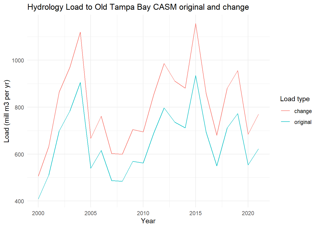
View the total annual hydrology load from before and with the change.

Code

toplo <- hydlydat |> 
  mutate(Year = year(date)) |> 
  summarise(
    original = sum(hy_load),
    change = sum(hy_load_chg), 
    .by = Year
  ) |> 
  pivot_longer(cols = c(original, change), names_to = 'var', values_to = 'load')

p <- ggplot(toplo, aes(x = Year, y = load, color = var)) +
  geom_line() +
  theme_minimal() + 
  labs(title = 'Hydrology Load to Old Tampa Bay CASM original and change',
       x = 'Year',
       y = 'Load (mill m3 per yr)',
       color = 'Load type')
p

Save Hydrology file

Save the hydrology data in the format received from SB.

Code

out <- hydlydat |> 
  mutate(
    year = year(date),
    month = month(date),
    bay_segment = 'Old Tampa Bay',
    Day = mday(date), 
    Count = 1:n()
  ) |> 
  mutate(
    year = ifelse(duplicated(year), "", year),
    month = ifelse(duplicated(month), "", month),
    bay_segment = ifelse(duplicated(bay_segment), "", bay_segment), 
    .by = c(year, month, bay_segment)
  ) |> 
  select(year, month, bay_segment, Date = date, Discharge_hy_load_106_m3_d = hy_load_chg, Count, Day)

write.csv(out, here::here('data-raw/OTB_hydro_daily-interpolated_chg.csv'))