Load projections all bay segments

Code

library(tidyverse)
library(sf)

load(file = here::here('data-raw/mosdat.RData'))
load(file = here::here('data-raw/mohydat.RData'))
load(file = here::here('data-raw/tnanndat.RData'))
load(file = here::here('data/allsubbas.RData'))

segs <- c('Old Tampa Bay', 'Hillsborough Bay', 'Middle Tampa Bay')

# monthly data
lddatmo <- mosdat |> 
  filter(bay_segment %in% segs) |> 
  filter(year >= 2000 & year <= 2021) |> 
  select(-bod_load) |> 
  summarise(
    tp_load = sum(tp_load), 
    tss_load = sum(tss_load),
    .by = c('year', 'month', 'bay_segment')
  ) |> 
  left_join(mohydat, by = c('year', 'month', 'bay_segment')) |> 
  pivot_longer(tp_load:hy_load_106_m3_mo, names_to = 'var', values_to = 'val')
npstnlddatmo <- mosdat |> 
  filter(bay_segment %in% segs) |> 
  filter(year >= 2000 & year <= 2021) |> 
  filter(source == 'NPS') |>
  mutate(var = c('tn_load')) |> 
  select(year, month, bay_segment, var, val = tn_load)
lddatmo <- lddatmo |> 
  bind_rows(npstnlddatmo) |> 
  mutate(
    bay_segment = factor(bay_segment, levels = segs),
    var = factor(var, levels = c('tn_load', 'tp_load', 'tss_load', 'hy_load_106_m3_mo'), 
                 labels = c('TN (NPS)', 'TP' ,'TSS', 'HY'))
  ) |>   
  arrange(year, month, bay_segment, var)

# annual data
lddatann <- lddatmo |> 
  summarise(
    val = sum(val), 
    .by = c('year', 'bay_segment', 'var')
  )

This document shows a projection of estimated load change to 2040 based on annual loading estimates from 2000 to 2021 for all bay segments, except LTB.

Estimating projections

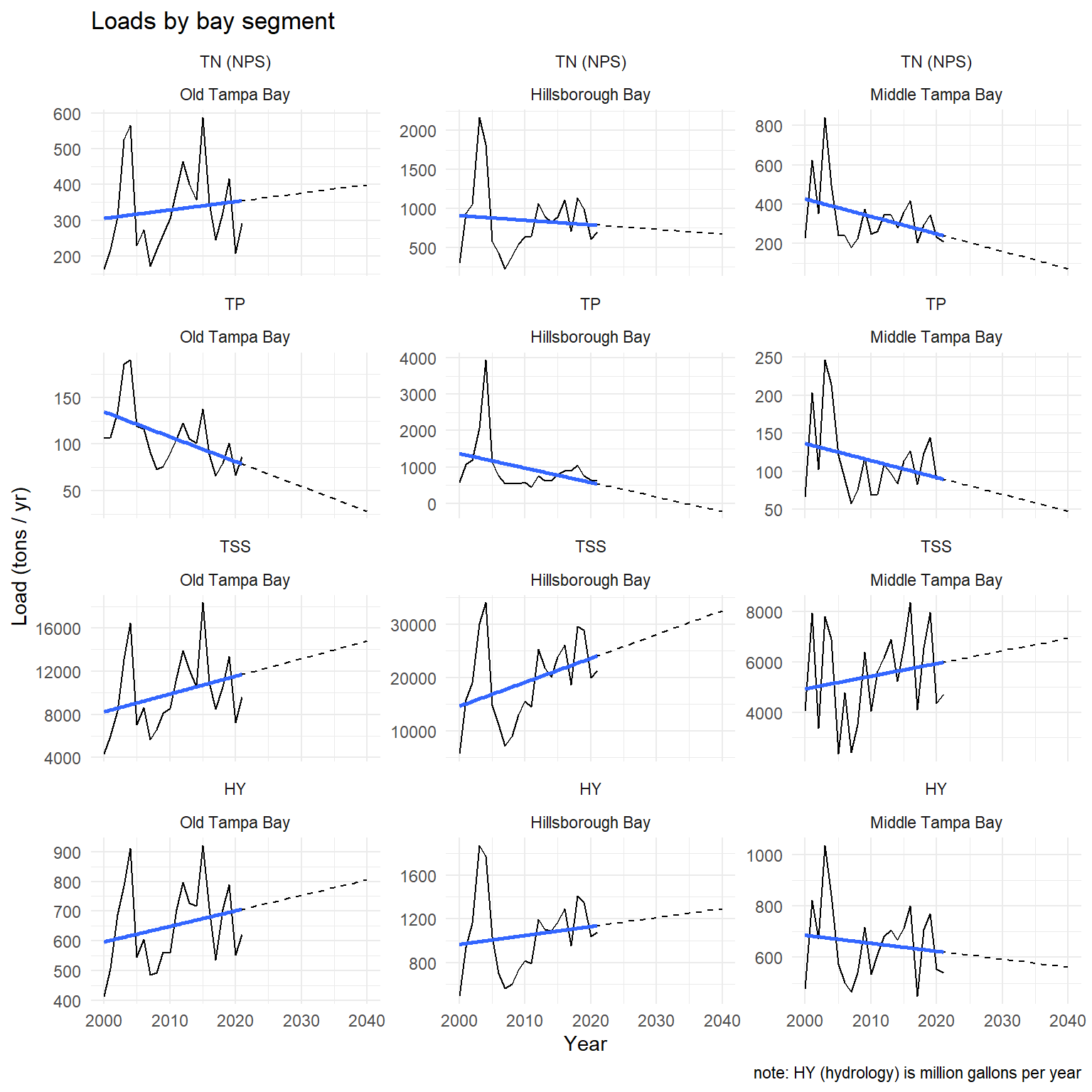
A regression fit is first made from 2000 to 2021 for each parameter and bay segment, then projected to 2040. Note that this is only done for NPS for TN. All other parameters use the combined load sources for the projection.

Code

# regression model of tn_load by year
mod <- lm(val ~ year*bay_segment*var, data = lddatann)

# get predictions for years 2000:2040
preds <- data.frame(year = 2000:2040) |> 
  crossing(
    bay_segment = factor(segs, levels = segs), 
    var = factor(levels(lddatann$var), levels = levels(lddatann$var))
  )
preds <- preds |> 
  mutate(
    val = predict(mod, preds)
  ) 

# plot tn_load as line plot by year
# add regression predictions
p <- ggplot(lddatann, aes(x = year, y = val)) +
  geom_line() +
  geom_line(data = preds, linetype = 'dashed') +
  geom_smooth(method = 'lm', se = F, formula = y ~ x) + 
  facet_wrap(var~bay_segment, ncol = 3, scales = 'free_y') + 
  labs(title = 'Loads by bay segment',
       x = 'Year',
       y = 'Load (tons / yr)',
       caption = 'note: HY (hydrology) is million gallons per year'
  ) +
  theme_minimal()
p

The percent change is calculated as the average value from the regression fit for 2000 to 2021 to 2040.

Code

# estimate means from 2000 to 2021 and 2040
means <- preds |> 
  summarise(
    mean_load_2000_2021 = mean(val[year >= 2000 & year <= 2021]),
    mean_load_2040 = mean(val[year == 2040]), 
    .by = c(bay_segment, var)
  )

# take percent change from 2000 to 2021 to 2040
means <- means |> 
  mutate(
    percent_change = (mean_load_2040 - mean_load_2000_2021) / mean_load_2000_2021 * 100, 
    .by = c(bay_segment, var)
  )
means

# A tibble: 12 × 5
   bay_segment      var      mean_load_2000_2021 mean_load_2040 percent_change
   <fct>            <fct>                  <dbl>          <dbl>          <dbl>
 1 Old Tampa Bay    TN (NPS)                330.          400.            21.0
 2 Old Tampa Bay    TP                      107.           27.9          -73.9
 3 Old Tampa Bay    TSS                    9973.        14812.            48.5
 4 Old Tampa Bay    HY                      651.          806.            23.7
 5 Hillsborough Bay TN (NPS)                849.          674.           -20.6
 6 Hillsborough Bay TP                      958.         -213.          -122. 
 7 Hillsborough Bay TSS                   19318.        32568.            68.6
 8 Hillsborough Bay HY                     1053.         1293.            22.8
 9 Middle Tampa Bay TN (NPS)                335.           72.8          -78.3
10 Middle Tampa Bay TP                      113.           47.5          -58.1
11 Middle Tampa Bay TSS                    5463.         6944.            27.1
12 Middle Tampa Bay HY                      654.          562.           -14.1

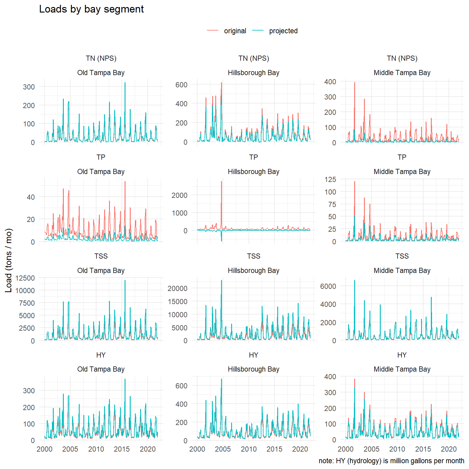
The estimated changes can then be projected onto to observed load values for 2000 to 2021. Note that some have negative projections due to extrapolation of the regression to values less than zero.

Code

lddatmochg <- lddatmo |> 
  left_join(means, by = c('bay_segment', 'var')) |> 
  select(-mean_load_2000_2021, -mean_load_2040) |> 
  mutate(
    valchg = val + (val * (percent_change / 100)), 
    date = make_date(year, month, '1')
  )

p <- ggplot(lddatmochg, aes(x = date)) +
  geom_line(aes(y = val, color = 'original')) +
  geom_line(aes(y = valchg, color = 'projected')) +
  facet_wrap(var~bay_segment, ncol = 3, scales = 'free_y') + 
  labs(title = 'Loads by bay segment',
       x = NULL,
       y = 'Load (tons / mo)', 
       color = NULL,
       caption = 'note: HY (hydrology) is million gallons per month'
  ) +
  theme_minimal() + 
  theme(legend.position = 'top')
p

Verify the percent change is correct. This should be the same as the means object.

Code

lddatmochg |> 
  summarize(
    val = sum(val),
    valchg = sum(valchg), 
    .by = c(bay_segment, var)
  ) |> 
  mutate(
    percent_change =  (valchg - val) / val * 100
  )

# A tibble: 12 × 5
   bay_segment      var          val  valchg percent_change
   <fct>            <fct>      <dbl>   <dbl>          <dbl>
 1 Old Tampa Bay    TN (NPS)   7266.   8795.           21.0
 2 Old Tampa Bay    TP         2348.    614.          -73.9
 3 Old Tampa Bay    TSS      219397. 325854.           48.5
 4 Old Tampa Bay    HY        14327.  17721.           23.7
 5 Hillsborough Bay TN (NPS)  18673.  14830.          -20.6
 6 Hillsborough Bay TP        21068.  -4682.         -122. 
 7 Hillsborough Bay TSS      424994. 716495.           68.6
 8 Hillsborough Bay HY        23157.  28436.           22.8
 9 Middle Tampa Bay TN (NPS)   7365.   1602.          -78.3
10 Middle Tampa Bay TP         2493.   1045.          -58.1
11 Middle Tampa Bay TSS      120193. 152766.           27.1
12 Middle Tampa Bay HY        14395.  12366.          -14.1

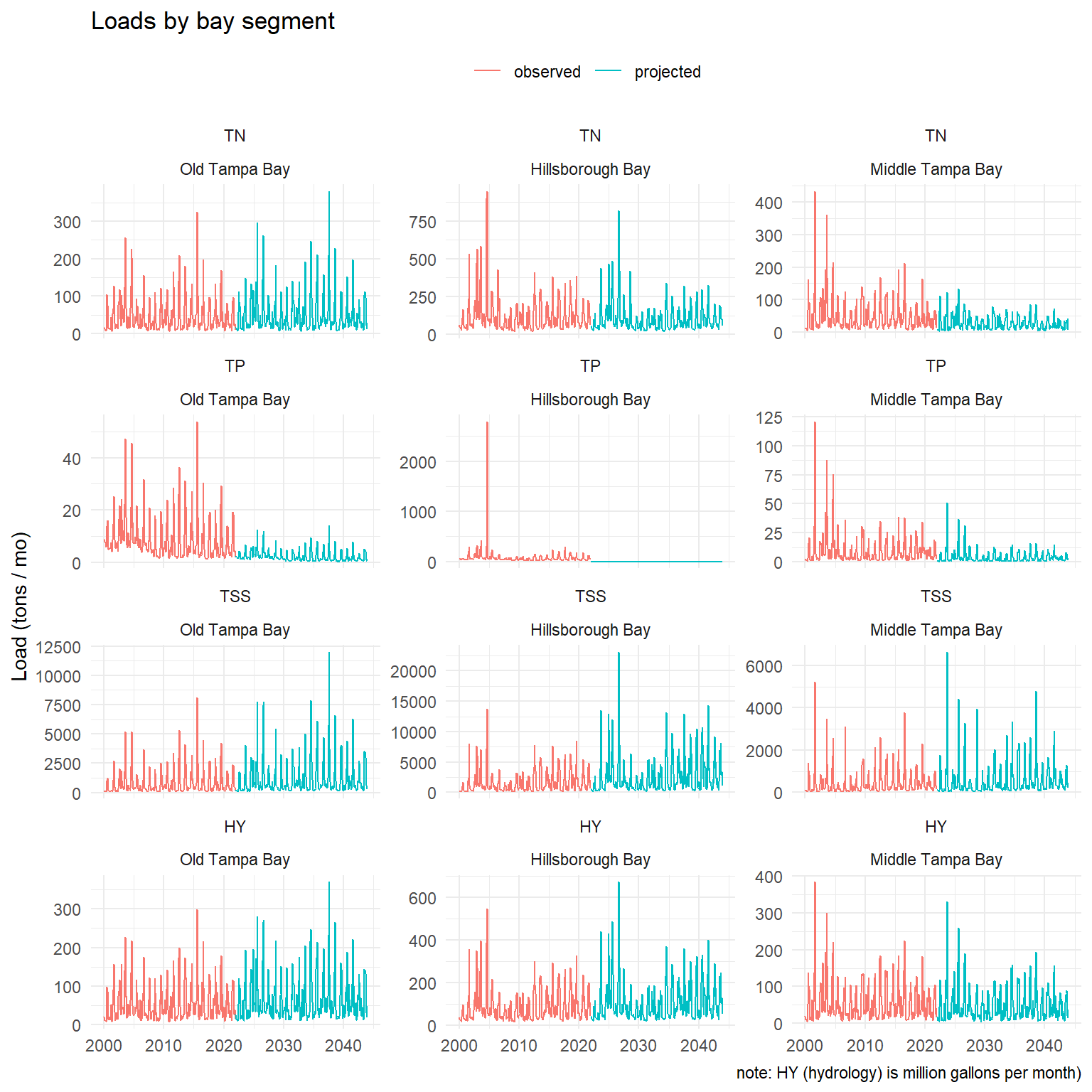
The last step is to add the NPS change for TN to the total TN load and assign the projected values to the next twenty years. Projected values are also floored at zero.

Code

tnnpsmochg <- lddatmochg |> 
  filter(var == 'TN (NPS)') |> 
  select(year, month, bay_segment, valchg)
tnmodat <- mosdat |> 
  filter(year >= 2000 & year <= 2021) |> 
  filter(bay_segment %in% segs) |> 
  select(-tp_load, -tp_load, -tss_load, -bod_load) |> 
  left_join(tnnpsmochg, by = c('year', 'month', 'bay_segment')) |> 
  mutate(
    valchg = case_when(
      source == 'NPS' ~ valchg, 
      T ~ tn_load
    ),
    var = 'TN',
    bay_segment = factor(bay_segment, levels = segs)
  ) |> 
  summarise(
    val = sum(tn_load),
    valchg = sum(valchg),
    .by = c(year, month, bay_segment, var)
  )
projected <- lddatmochg |> 
  filter(var != 'TN (NPS)') |> 
  select(year, month, bay_segment, var, val, valchg) |> 
  bind_rows(tnmodat) |> 
  mutate(var = factor(var, levels = c('TN', 'TP', 'TSS', 'HY'))) |> 
  pivot_longer(c(val, valchg), names_to = 'period', values_to = 'val') |> 
  mutate(
    year = case_when(
      period == 'valchg' ~ year + 22, 
      T ~ year
    ),
    date = make_date(year, month, '1'), 
    period = factor(period, levels = c('val', 'valchg'), labels = c('observed', 'projected')),
    val = pmax(val, 0)
  ) |> 
  arrange(date, bay_segment, var)

p <- ggplot(projected, aes(x = date, y = val, color = period)) +
  geom_line() +
  facet_wrap(var~bay_segment, ncol = 3, scales = 'free_y') + 
  labs(title = 'Loads by bay segment',
       x = NULL,
       y = 'Load (tons / mo)', 
       color = NULL,
       caption = 'note: HY (hydrology) is million gallons per month)'
  ) +
  theme_minimal() + 
  theme(legend.position = 'top')
p

Assigning to model segments

There are three model segments for OTB, two for HB, and three for MTB. The loads are apportioned in to equal amounts based on the number of model segments per segment, except OTB which uses amounts described here. The previous link assigns values to NW, NE, CW, CE, SW, and SE sub-segments as sixths, which are assigned to model segments 1, 2, and 3 as NW/NE, CW/CE, and SW/SE. Here we simply apportion using the relative areas that drain to each OTB subsegment, whereas the previous example used a hydrologic basin dataset from 2017-2021 that had gaged and ungaged loading estimates.

Code

otbprop <- allsubbas |> 
  mutate(
    acres = units::set_units(st_area(allsubbas), 'acres'), 
    modelseg = case_when(
      subsegment %in% c('NW', 'NE') ~ 1, 
      subsegment %in% c('CW', 'CE') ~ 2, 
      subsegment %in% c('SW', 'SE') ~ 3
    )
  ) |> 
  st_set_geometry(NULL) |> 
  group_by(modelseg) |> 
  summarise(
    acres = sum(acres)
  ) |> 
  mutate(
    bay_segment = 'Old Tampa Bay',
    prop = as.numeric(acres / sum(acres))
  ) |> 
  select(-acres)

allprop <- tibble(
    modelseg  = c(4:8),
    bay_segment = c(rep('Hillsborough Bay', 2), rep('Middle Tampa Bay', 3)),
    prop = c(rep(0.5, 2), rep(1/3, 3))
  ) |> 
  bind_rows(otbprop) |> 
  mutate(bay_segment = factor(bay_segment, levels = segs)) |> 
  arrange(bay_segment)
allprop

# A tibble: 8 × 3
  modelseg bay_segment        prop
     <dbl> <fct>             <dbl>
1        1 Old Tampa Bay    0.766 
2        2 Old Tampa Bay    0.176 
3        3 Old Tampa Bay    0.0580
4        4 Hillsborough Bay 0.5   
5        5 Hillsborough Bay 0.5   
6        6 Middle Tampa Bay 0.333 
7        7 Middle Tampa Bay 0.333 
8        8 Middle Tampa Bay 0.333

The allprop object is joined to the observed and projected monthly loads by bay segment and then the loads are multiplied by the proportions.

Code

out <- allprop |> 
  left_join(projected, by = 'bay_segment', relationship = c('many-to-many')) |> 
  mutate(val = val * prop)
out

# A tibble: 16,896 × 9
   modelseg bay_segment    prop  year month var   period     val date      
      <dbl> <fct>         <dbl> <dbl> <dbl> <fct> <fct>    <dbl> <date>    
 1        1 Old Tampa Bay 0.766  2000     1 TN    observed 12.3  2000-01-01
 2        1 Old Tampa Bay 0.766  2000     1 TP    observed  6.88 2000-01-01
 3        1 Old Tampa Bay 0.766  2000     1 TSS   observed 94.4  2000-01-01
 4        1 Old Tampa Bay 0.766  2000     1 HY    observed 16.0  2000-01-01
 5        1 Old Tampa Bay 0.766  2000     2 TN    observed  9.63 2000-02-01
 6        1 Old Tampa Bay 0.766  2000     2 TP    observed  6.38 2000-02-01
 7        1 Old Tampa Bay 0.766  2000     2 TSS   observed 79.8  2000-02-01
 8        1 Old Tampa Bay 0.766  2000     2 HY    observed  9.12 2000-02-01
 9        1 Old Tampa Bay 0.766  2000     3 TN    observed  8.42 2000-03-01
10        1 Old Tampa Bay 0.766  2000     3 TP    observed  6.19 2000-03-01
# ℹ 16,886 more rows

Now verify that the totals are the same between the model segment assigned dataset and the original.

Code

summarise(out, val = sum(val), .by = c(bay_segment, var))

# A tibble: 12 × 3
   bay_segment      var        val
   <fct>            <fct>    <dbl>
 1 Old Tampa Bay    TN      26378.
 2 Old Tampa Bay    TP       2962.
 3 Old Tampa Bay    TSS    545251.
 4 Old Tampa Bay    HY      32049.
 5 Hillsborough Bay TN      60698.
 6 Hillsborough Bay TP      21068.
 7 Hillsborough Bay TSS   1141488.
 8 Hillsborough Bay HY      51593.
 9 Middle Tampa Bay TN      20821.
10 Middle Tampa Bay TP       3538.
11 Middle Tampa Bay TSS    272960.
12 Middle Tampa Bay HY      26761.

Code

summarise(projected, val = sum(val), .by = c(bay_segment, var))

# A tibble: 12 × 3
   bay_segment      var        val
   <fct>            <fct>    <dbl>
 1 Old Tampa Bay    TN      26378.
 2 Old Tampa Bay    TP       2962.
 3 Old Tampa Bay    TSS    545251.
 4 Old Tampa Bay    HY      32049.
 5 Hillsborough Bay TN      60698.
 6 Hillsborough Bay TP      21068.
 7 Hillsborough Bay TSS   1141488.
 8 Hillsborough Bay HY      51593.
 9 Middle Tampa Bay TN      20821.
10 Middle Tampa Bay TP       3538.
11 Middle Tampa Bay TSS    272960.
12 Middle Tampa Bay HY      26761.

Code

write.csv(out, here::here('data-raw/boxmodproject.csv'), row.names = F)