Code
# turn off all chunks by default
knitr::opts_chunk$set(eval = FALSE)Themes for indicators seeking relevance to:
Icons
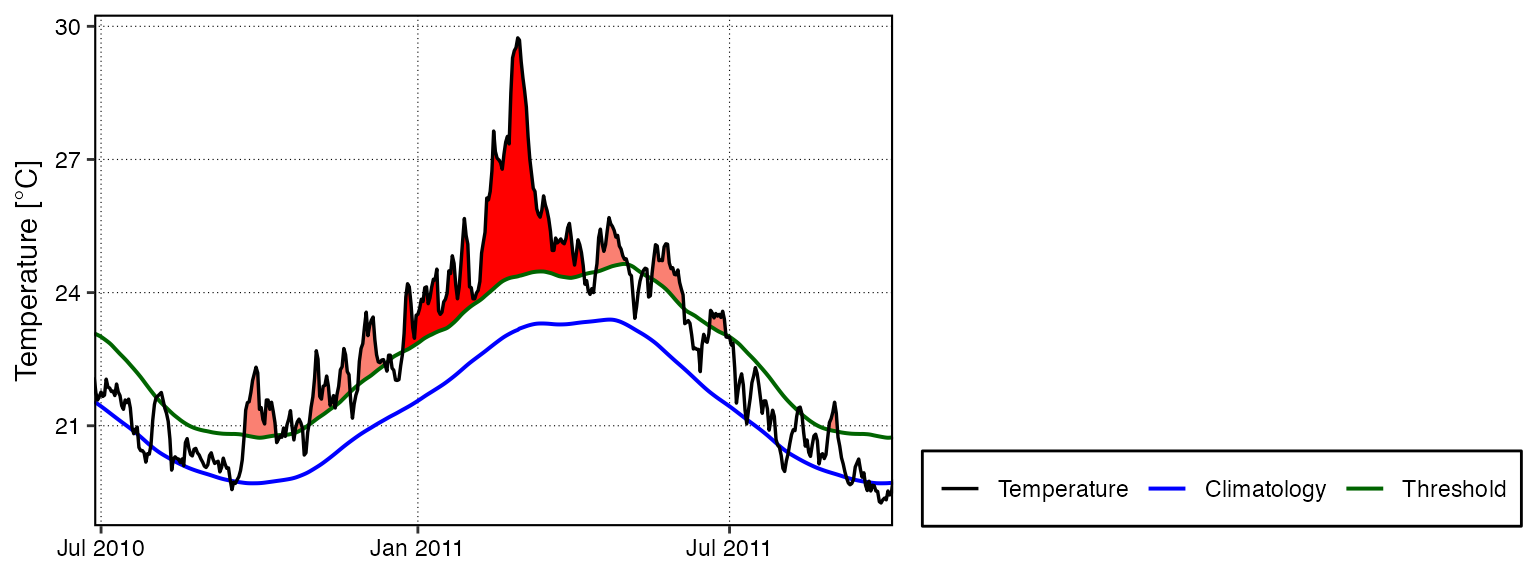
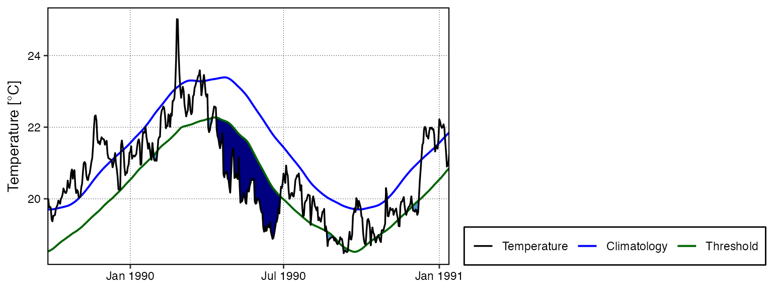
Data descriptive of the risks of climate change can be obtained from several sources. These may include weather or climatological data, long-term tidal gauge data, or in situ water measurements responsive to climate change. Weather and climatological data could be obtained from local weather stations with long-term data, e.g., Tampa International Airport, and could include measures of air temperature, precipitation, and/or storm intensity/frequency. Tidal gauge data are readily available from the NOAA PORTS data retrieval system. Lastly, in situ water measurements could include water temperature, changes in flow hydrology, salinity, and/or pH. Data used to evaluate potential risks related to ocean acidification should also be explored.
The permanency and ease of access of each data source should be noted when making recommendations on indicators to operationalize. Further, indicators that communicate the risks associated with climate change are preferred, as opposed to those that simply indicate change. An example is the number of days in a year when temperature exceeds a critical threshold, as compared to temperature alone. An additional example is frequency of sunny day flooding events, as compared to tidal gauge measurements alone.
# turn off all chunks by default
knitr::opts_chunk$set(eval = FALSE)# options(repos=c(CRAN="https://cran.mirror.garr.it/CRAN/"))
# install.packages(c("sf","terra"), type = "binary")
# renv::snapshot()
# renv::clean()
# renv::rebuild()
# built from source: sp, survival, rnoaa, tbeptools
if (!"librarian" %in% rownames(installed.packages()))
install.packages("librarian")
librarian::shelf(
dplyr, dygraphs, glue, here, htmltools, leaflet, leaflet.extras2, lubridate,
sf, stringr, tbep-tech/tbeptools, prism, purrr,
RColorBrewer, readr, rnoaa, terra, tidyr, webshot2,
quiet = T)
# explicitly list packages for renv::dependencies(); renv::snapshot()
library(dplyr)
library(dygraphs)
library(glue)
library(here)
library(leaflet)
library(librarian)
library(lubridate)
library(RColorBrewer)
library(prism)
library(purrr)
library(readr)
library(rnoaa)
library(sf)
library(stringr)
library(tbeptools)
library(terra)
library(tidyr)
library(webshot2)
options(readr.show_col_types = F)noaacrwsstDaily
The rnoaa R package uses NOAA NCDC API v2, which only goes to 2022-09-15.
NCEI Web Services | Climate Data Online (CDO) | National Center for Environmental Information (NCEI)
Data Tools | Climate Data Online (CDO) | National Climatic Data Center (NCDC)
Got token at ncdc.noaa.gov/cdo-web/token. Added variable NOAA_NCDC_CDO_token to:
locally:
file.edit("~/.Renviron")on GitHub: Repository secrets in Actions secrets · tbep-tech/climate-change-indicators
PRCP: Precipitation (tenths of mm)TMAX: Maximum temperature (tenths of degrees C)TMIN: Minimum temperature (tenths of degrees C)# provide NOAA key
options(noaakey = Sys.getenv("NOAA_NCDC_CDO_token"))
# Specify datasetid and station
stn <- "GHCND:USW00012842" # TAMPA INTERNATIONAL AIRPORT, FL US
stn_csv <- here("data/tpa_ghcnd.csv")
stn_meta_csv <- here("data/tpa_meta.csv")
if (!file.exists(stn_meta_csv)){
# cache station metadata since timeout from Github Actions
stn_meta <- ncdc_stations(
datasetid = "GHCND",
stationid = stn)
write_csv(stn_meta$data, stn_meta_csv)
}
read_csv(stn_meta_csv)
if (!file.exists(stn_csv)){
date_beg <- stn_meta$data$mindate
date_end <- stn_meta$data$maxdate
max_rows <- 1000
vars <- c("PRCP","TMIN","TMAX")
n_vars <- length(vars)
days_batch <- floor(max_rows / n_vars)
dates <- unique(c(
seq(
ymd(date_beg),
ymd(date_end),
by = glue("{days_batch} days")),
ymd(date_end)))
n_i <- length(dates) - 1
for (i in 1:n_i){
# for (i in 14:n_i){
date_beg <- dates[i]
if (i == n_i){
date_end <- dates[i+1]
} else {
date_end <- dates[i+1] - days(1)
}
print(glue("{i} of {n_i}: {date_beg} to {date_end} ~ {Sys.time()}"))
# retry if get Error: Service Unavailable (HTTP 503)
o <- NULL
attempt <- 1
attempt_max <- 10
while (is.null(o) && attempt <= attempt_max) {
if (attempt > 1)
print(glue(" attempt {attempt}", .trim = F))
attempt <- attempt + 1
try(
o <- ncdc(
datasetid = "GHCND",
stationid = stn,
datatypeid = vars,
startdate = date_beg,
enddate = date_end,
limit = max_rows) )
}
if (i == 1) {
df <- o$data
} else {
df <- rbind(df, o$data)
}
}
stopifnot(duplicated(df[,1:2])|> sum() == 0)
df <- df |>
mutate(
date = as.Date(strptime(
date, "%Y-%m-%dT00:00:00")),
datatype = recode(
datatype,
PRCP = "precip_mm",
TMIN = "temp_c_min",
TMAX = "temp_c_max"),
value = value / 10) |>
select(
-station, # station : all "GHCND:USW00012842"
-fl_m, # measurement flag: 3,524 are "T" for trace
-fl_t, # time flag: all "2400"
-fl_q) # quality flag: all ""
write_csv(df, stn_csv)
}
d <- read_csv(stn_csv)
d |>
select(date, datatype, value) |>
filter(datatype %in% c("temp_c_min","temp_c_max")) |>
pivot_wider(
names_from = datatype,
values_from = value) |>
dygraph(main = "Daily Temperature (ºC)") |>
dyOptions(
colors = brewer.pal(5, "YlOrRd")[c(5,3)]) |>
dySeries("temp_c_min", label = "min") |>
dySeries("temp_c_max", label = "max")
d |>
select(date, datatype, value) |>
filter(datatype %in% c("precip_mm")) |>
pivot_wider(
names_from = datatype,
values_from = value) |>
dygraph(main = "Daily Precipitation (mm)") |>
dySeries("precip_mm", label = "precip")TODO: - trend analysis. e.g. NOAA’s Climate at a Glance. Typically based on the last 30 years, but here we’ve got back to 1939-02-01 so almost 100 years. Keep it 5 years and see how rate changing over time.
Materials:
“RAIN AS A DRIVER” in tbep-os-presentations/state_of_the_bay_2023.qmd
Precipitation - NEXRAD QPE CDR | National Centers for Environmental Information (NCEI)
librarian::shelf(
  dplyr, here, leaflet,
  # mapview,
  readxl, sf, tbep-tech/tbeptools)
# register with renv
library(dplyr)
library(here)
library(leaflet)
# library(mapview)
library(readxl)
library(sf)
library(tbeptools)

# from SWFWMD grid cells, use only if interested in areas finer than TB watershed
# this currently gets the same data as the compiled spreadsheet
grd <- st_read(here('../tbep-os-presentations/data/swfwmd-GARR-gisfiles-utm/swfwmd_pixel_2_utm_m_83.shp'), quiet = T)
# mapView(grd)

tbgrdcent <- grd %>%
  st_transform(crs = st_crs(tbshed)) %>%
  st_centroid() %>%
  .[tbshed, ]

# unzip folders
loc <- here('../tbep-os-presentations/data/swfwmd_rain')
# files <- list.files(loc, pattern = '.zip', full.names = T)
# lapply(files, unzip, exdir = loc)

# read text files
raindat <- list.files(loc, pattern = '19.*\\.txt$|20.*\\.txt$', full.names = T) %>%
  lapply(read.table, sep = ',', header = F) %>%
  do.call('rbind', .) %>%
  rename(
    'PIXEL' = V1,
    'yr' = V2,
    'inches' = V3) %>%
  filter(PIXEL %in% tbgrdcent$PIXEL)

# ave rain dat
raindatave <- raindat %>%
  summarise(
    inches = mean(inches, na.rm = T),
    .by = 'yr')

##
# use compiled SWFWMD data

# # https://www.swfwmd.state.fl.us/resources/data-maps/rainfall-summary-data-region
# # file is from the link "USGS watershed"
# download.file(
#   'https://www4.swfwmd.state.fl.us/RDDataImages/surf.xlsx?_ga=2.186665249.868698214.1705929229-785009494.1704644825',
#   here('data/swfwmdrainfall.xlsx'),
#   mode = 'wb'
#   )

raindatave_url <- "https://www4.swfwmd.state.fl.us/RDDataImages/surf.xlsx"
dir.create(here('data/swfwmd.state.fl.us'))
raindatave_xl <- here('data/swfwmd.state.fl.us/surf.xlsx')

download.file(raindatave_url, raindatave_xl)
read_excel(raindatave_xl)

download.file(raindatave_url, here('data/swfwmdrainfall.xlsx'), mode = 'wb')

raindatave <- read_excel(
  raindatave_xl, sheet = 'ann-usgsbsn', skip = 1) %>%
  filter(Year %in% 1975:2023) %>%
  select(
    yr = Year,
    inches = `Tampa Bay/Coastal Areas`
  ) %>%
  mutate_all(as.numeric)

raindatave_now <-
readxl::read_excel()

raindatave <- read_excel(here('data/swfwmdrainfall.xlsx'), sheet = 'ann-usgsbsn', skip = 1) %>%
  filter(Year %in% 1975:2023) %>%
  select(
    yr = Year,
    inches = `Tampa Bay/Coastal Areas`
  ) %>%
  mutate_all(as.numeric)

# ave chldat
chlave <- anlz_avedat(epcdata) %>%
  .$ann %>%
  filter(var == 'mean_chla') %>%
  summarise(
    chla = mean(val, na.rm = T),
    .by = 'yr'
  ) %>%
  filter(yr >= 1975)

toplo <- inner_join(chlave, raindatave, by = 'yr')

p1 <- ggplot(raindatave, aes(x = yr, y = inches)) +
  geom_line() +
  geom_point() +
  geom_point(data = raindatave[chlave$yr == 2023, ], col = 'red', size = 2) +
  theme_minimal() +
  theme(
    panel.grid.minor = element_blank(),
  ) +
  labs(
    x = NULL,
    y = 'Annual rainfall (inches)',
    title = 'Annual rainfall',
    subtitle = 'Tampa Bay watershed, 1975 - 2023'
  )

p2 <- ggplot(chlave, aes(x = yr, y = chla)) +
  geom_line() +
  geom_point() +
  geom_point(data = chlave[chlave$yr == 2023, ], col = 'red', size = 2) +
  theme_minimal() +
  theme(
    panel.grid.minor = element_blank(),
  ) +
  labs(
    x = NULL,
    y = 'Chlorophyll-a (ug/L)',
    title = 'Annual mean chlorophyll-a',
    subtitle = 'All segments, 1975 - 2023'
  )

p3 <- ggplot(toplo, aes(x = inches, y = chla)) +
  geom_text_repel(aes(label = yr), point.size = NA, segment.size = NA) +
  geom_label_repel(data = toplo[toplo$yr == 2023, ], aes(label = yr), color = 'red', point.size = NA) +
  geom_smooth(formula = y ~ x, method = 'lm', se = F, color = 'red') +
  # geom_segment(aes(x = 45, xend = 40, y = 4.86, yend = 4.86), color = 'red', arrow = arrow(length = unit(0.2, "inches")), linewidth = 1) +
  theme_minimal() +
  theme(
    panel.grid.minor = element_blank(),
  ) +
  labs(
    x = 'Annual rainfall (inches)',
    y = 'Chlorophyll-a (ug/L)',
    title = 'Annual mean chlorophyll-a vs. rainfall',
    caption = 'Data from EPCHC, SWFWMD'
  )

p <- (p1 / p2) | p3
p# librarian::shelf(rNOMADS)The Parameter-elevation Relationship on Independent Slopes Model (PRISM) is a combined dataset consisting of ground gauge station and RADAR products. The data is on a 4km grid resolution covering the contiguous United States. Data is available from 1981 to present.PRISM data are reported in GMT (UTC). PRISM provides daily average temperature and dew-point temperature data. Relative humidity is calculated using a version of the August-Roche-Magnus equation as follows ):
RH = 100*(EXP((17.625*TD)/(243.04+TD))/EXP((17.625*T)/(243.04+T)))where,RHis % relative humidity,TDis dew-point temperature (celsius), andTis air temperature (celsius).
“Normal” precipitation is derived from PRISM climate data, created at Oregon State University. The PRISM gridded climate maps are considered the most detailed, highest-quality spatial climate datasets currently available.
prism R package
| Parameter | Description |
|---|---|
tmin |
Minimum temperature |
tmax |
Maximum temperature |
tmean |
Mean temperature (tmean == mean(tmin, tmax)) |
tdmean |
Mean dew point temperature |
ppt |
Total precipitation (rain and snow) |
vpdmin |
Daily minimum vapor pressure deficit |
vpdmax |
Daily maximum vapor pressure deficit |
Data are at 4km resolution, except for the normals which can also be downloaded at 800m resolution.
Temporal data availability:
Recent
1981 to present
daily, monthly, annual data
Historical
1895 through 1980
complete monthly and annual data by year
Normals
30-year normals daily, monthly, and annual normals, each as a single grid The 30 year PRISM normal from 1981-2010 is used for precipitation analysis since 2004. Prior to 2004 the 30 year PRISM normal from 1961-1990 is used.
Forms
stable
provisional
early
Daily data are considered “early” for the current month. The previous six months are provisional data. After six months data are considered stable. Thus early data only exist for daily data, while there can be monthly (and presumably yearly) provisional data. –
?prism::prism_archive_clean
tbeptools::read_importprism()@example from tbeptools::read_importprism()# devtools::install_local("../tbeptools", force = T)
# devtools::load_all("../tbeptools")
# setup output directory and table
dir_tif <- here::here("../tbeptools/inst/prism")
zonal_csv <- file.path(dir_tif, "_zones.csv")
# run function for Tampa Bay watersheds for first 3 days and 4 variables
d <- read_importprism(
vars = c("tmin", "tmax", "tdmean", "ppt"),
date_beg = as.Date("1981-01-01"),
date_end = as.Date("1981-01-03"),
dir_tif = dir_tif,
sf_zones = tbsegshed,
fld_zones = "bay_segment",
zonal_csv = zonal_csv)
# plot first of output rasters
tifs <- list.files(dir_tif, pattern = ".tif$", full.names = T)
basename(tifs)
r <- terra::rast(tifs[1])
names(r) # {data observed}_{variable}_v{version}_{date updated}
terra::plet(
r[[3]],
main = names(r)[3],
col = "Spectral",
tiles = "CartoDB.DarkMatter")
# show summary by zone
dlibrarian::shelf(
dplyr, here, sf, tbep-tech/tbeptools)
# outputs
dir_prism <- here("data/prism")
prism_csv <- here("data/prism.csv")
# Tampa Bay watershed zones, including whole bay ("TB")
tb_zones <- tbsegshed |>
bind_rows(
tbshed |>
mutate(bay_segment = "TB") |>
select(bay_segment, geometry))
# bounding box with 0.2º margin around watershed, rounded to .1
bb <- tbshed |>
st_buffer(0.2) |>
st_bbox() |>
round(1)
# c(xmin = -82.9, ymin = 27.4, xmax = -81.9, ymax = 28.4)
# after running terra::trim() on raster:
bb <- c(xmin = -82.9, ymin = 27.2, xmax = -81.7, ymax = 28.6)
d <- read_importprism(
vars = c("tmin", "tmax", "tdmean", "ppt"),
date_beg = as.Date("1981-01-01"),
date_end = Sys.Date(),
bbox = bb,
dir_tif = dir_prism,
sf_zones = tb_zones,
fld_zones = "bay_segment",
zonal_csv = prism_csv,
verbose = T)
# show summary by zone
dTODO: Github Action on daily cron to run read_importprism() for all days and variables
# Get monthly (every month) and annual 30-year normals for precipitation

# get_prism_normals(

# type = "ppt",

# resolution = "800m",

# mon = 1:12,

# annual = TRUE,

# keepZip = FALSE)

var    <- "tmax"
period <- "daily"
date   <- today() - days(1) # yesterday

get_prism_dailys(
  type    = "tmax",
  dates   = date,
  keepZip = F)

pd <- prism_archive_subset(var, period, dates = date)
pd_image(pd, col="redblue")
r <- pd_stack(pd) |>
  rast()
plot(r)

library(leaflet)
r_3857 <- projectRasterForLeaflet(
  r, method = "bilinear")
pal <- colorNumeric(
  "Spectral",  values(r_3857, na.rm=T),
  na.color = "transparent")

leaflet() |>
  addProviderTiles(
    providers$CartoDB.Positron) |>
  addRasterImage(
    r_3857, opacity = 0.7) |>
  addPolygons(
    data = tbsegshed,
    fillOpacity = 0,
color = "purple", weight = 5)# tbshed_pd <- tbshed |>
r <- pd_stack(prism_archive_subset("tmax", "daily")[1])
crs <- crs(r, proj=T) # +proj=longlat +datum=NAD83 +no_defs
tbshed_pd <- tbsegshed |>
st_transform()
sf_use_s2(F)
tbshed_buf <- tbshed_pd |>
st_union() |>
st_make_valid() |>
st_buffer(0.2) |>
st_bbox() |>
st_as_sfc() |>
st_as_sf()
bb <- st_bbox(tbshed_buf) |> round(1)
# xmin ymin xmax ymax
# -83.1 27.2 -81.7 28.6
bb <- c(xmin = -83.1, ymin = 27.2, xmax = -81.7, ymax = 28.6)
ply_bb <- st_bbox(bb, crs = crs(r, proj=T)) |>
st_as_sfc() |>
st_as_sf()
leaflet() |>
addProviderTiles(providers$Stadia.StamenTonerLite) |>
addPolygons(data = ply_bb, color="green") |>
addPolygons(data = tbshed_pd)library(dplyr)
library(furrr) # install.packages("furrr")
library(glue)
library(here)
library(lubridate)
library(prism)
library(purrr)
library(sf)
library(terra)
n_cores <- parallel::detectCores() - 1
plan(multisession, workers = n_cores)
prism_archive_crop <- function(
type, temp_period, ...,
bb = c(xmin = -82.9, ymin = 27.2, xmax = -81.7, ymax = 28.6),
crs = "+proj=longlat +datum=NAD83 +no_defs", # WRONG: "+proj=longlat +ellps=GRS80 +no_defs"
verbose = F){
ply_bb <- sf::st_bbox(bb, crs = crs) |>
sf::st_as_sfc() |>
sf::st_as_sf()
pds <- prism::prism_archive_subset(type, temp_period, ...)
for (i in 1:length(pds)){ # i = 1
r <- prism::pd_stack(pds[i]) |>
terra::rast()
is_cropped <- all(sf::st_bbox(r) |> round(1) == bb)
if (!is_cropped){
r_bil <- terra::sources(r)
r_bb <- terra::crop(r, ply_bb, mask = T, touches = T) |>
terra::trim()
terra::writeRaster(r_bb, r_bil, filetype = "EHdr", overwrite = T)
bb_cropped <- sf::st_bbox(r_bb) |> round(1)
if (!all(bb_cropped == bb))
warning(glue(
"bbox of clipped raster rounded to 1 decimal:
{paste(bb_cropped, collapse=', ')}
does not match input argument `bb`:
{paste(bb, collapse=', ')}"))
}
}
}
yrs <- 1981:year(now())
mos <- 1:12
vars <- c("tmin", "tmax", "tdmean", "ppt")
# skipping: "tmean" [avg(tmin,tmax)], vapor pressure ["vpdmin", "vpdmax"]
# ((today() - days(1)) - date("1981-01-01")) |> as.integer() * length(vars) # 63,304 dirs expected in tmp/prism
n_dirs <- fs::dir_ls(here::here("tmp/prism"), type = "directory") |> length()
message(glue::glue("{n_dirs} ~ {Sys.time()}"))
# 1540 ~ 2024-05-02 18:28:41.717828
# 2527 ~ 2024-05-02 18:46:32.97783
# 3357 ~ 2024-05-02 18:59:52.753584
n_all <- 63304
n1 <- 1540
t1 <- parse_date_time(
"2024-05-02 18:28:41.717828", "Ymd HMS")
n2 <- 3357
t2 <- parse_date_time(
"2024-05-02 18:59:52.753584", "Ymd HMS")
dt <- difftime(t2, t1, units = "secs") |> as.integer()
dn <- n2 - n1
n_togo <- n_all - n2
eta <- t2 + seconds(dn / dt * n_togo)
message(glue::glue("ETA: {eta}"))
# ETA: 2024-05-03 10:20:03.1543
# ETA: 2024-05-03 11:10:09.588966
prism_set_dl_dir(here::here("tmp/prism"))
yesterday <- today() - days(1)
d_ymv = tibble(
yr = yrs) |>
cross_join(
tibble(mo = mos)) |>
cross_join(
tibble(var = vars)) |>
mutate(
date_beg = map2_chr(yr, mo, \(yr, mo){
date(glue("{yr}-{mo}-01")) |>
as.character() }),
date_end = map_chr(date_beg, \(date_beg){
# date_beg <- "2024-05-01"
date_end <- (date(date_beg) + months(1)) - days(1)
if (date_end > yesterday)
date_end <- yesterday
date_end |>
as.character()
}) ) |>
filter(date(date_beg) <= yesterday) |>
arrange(date_beg, date_end, var) |>
select(date_beg, date_end, var) |>
# filter(date(date_beg) >= date("1981-03-01")) |>
# rstudio.marinesensitivity.org:
# filter(
# date(date_beg) >= date("1981-09-01"),
# date(date_end) < date("1986-07-01")) # |>
# laptop:
# filter(
# date(date_beg) >= date("1986-12-01")) # |>
mutate(
n_files = pmap_int(list(
date_beg = date_beg,
date_end = date_end,
var = var), \(date_beg, date_end, var){
prism::prism_archive_subset(
var, "daily",
minDate = date_beg,
maxDate = date_end) |>
length() }),
n_days = map2_int(date_beg, date_end, \(date_beg, date_end){
difftime(date(date_end), date(date_beg), units = "days") |>
as.integer() }),
pct_done = n_files / n_days)
prism_csv <- here("tmp/prism.csv")
readr::write_csv(d_ymv, prism_csv)
# TODO: delete all extraneous station files
# find . -name "*_bil.stn.csv" -type f -delete
# TODO: on server remove dir
# dir='PRISM_ppt_provisional_4kmD2_20231101_bil'
# re='PRISM_(.*)_(.*)_(.*)_(.*)_bil'
# [[ $dir =~ $re ]] && date="${BASH_REMATCH[4]}" && echo "date: $date for $dir"
# var=${dir//$re/\1}
# type=${dir//$re/\2}
# res=${dir//$re/\3}
# date=${dir//$re/\4}
future_pmap(d_ymv, \(date_beg, date_end, var){
prism_set_dl_dir(here::here("tmp/prism"))
# fetch PRISM national rasters
get_prism_dailys(
type = var,
minDate = date_beg,
maxDate = date_end,
keepZip = F)
# remove any duplicates: stable > provisional > early
prism_archive_clean(
var, "daily",
minDate = date_beg,
maxDate = date_end)
# trim rasters to bounding box
prism_archive_crop(
var, "daily",
minDate = date_beg,
maxDate = date_end)
})
# clear future processes
if (!inherits(plan(), "sequential")) plan(sequential)prism_set_dl_dir(here::here("tmp/prism"))
for (var in vars)
prism_archive_crop(var, "daily")library(furrr) # install.packages("furrr")
n_cores <- parallel::detectCores() - 1
plan(multisession, workers = n_cores)
dir_prism <- here::here("tmp/prism")
prism_set_dl_dir(dir_prism)
vars <- c("tmin", "tmax", "tdmean", "ppt")
dates_all <- (date("1981-01-01"):(today() - days(1))) |> as.Date()
rx <- "PRISM_(.*)_(.*)_(.*)_(.*)_bil"
d_done <- tibble()
for (var in vars){ # var <- vars[4]
pds <- prism::prism_archive_subset(type = var, temp_period = "daily")
d_var <- tibble(
pd = pds) |>
mutate(
var = str_replace(pd, rx, "\\1"),
class = str_replace(pd, rx, "\\2"),
date = str_replace(pd, rx, "\\4") |>
as.Date(format = "%Y%m%d") )
if (nrow(d_done) == 0){
d_done <- d_var
} else {
d_done <- d_done |>
bind_rows(d_var)
}
}
# table(d_done$var)
# ppt tdmean tmax tmin
# 15759 15807 15746 15805
d_todo <- tibble(
var = vars) |>
cross_join(tibble(
date = dates_all)) |>
anti_join(
d_done |>
select(var, date),
by = c("date", "var"))
prism_dates_crop <- function(
var,
dates,
dir_prism = here::here("tmp/prism")){
# var = "tmin"; dates = date("2024-05-01"); dir_prism = here::here("tmp/prism")
# PRISM_tmin_early_4kmD2_20240509_bil
# ls -l | grep -v stable | grep -v provisional | tail
# ls -l | grep tmin_stable | head : PRISM_tmin_stable_4kmD2_19810101_bil
# ls -l | grep tmin_stable | tail : PRISM_tmin_stable_4kmD2_20231031_bil
# ls -l | grep tmin_provisional | head : PRISM_tmin_provisional_4kmD2_20231101_bil
# ls -l | grep tmin_provisional | tail : PRISM_tmin_provisional_4kmD2_20240430_bil
# ls -l | grep tmin_early | head : PRISM_tmin_early_4kmD2_20240501_bil
# ls -l | grep tmin_early | tail : PRISM_tmin_early_4kmD2_20240509_bil
# rm -r PRISM_tmin_stable_4kmD2_19810101_bil \
# PRISM_tmin_stable_4kmD2_20231031_bil \
# PRISM_tmin_provisional_4kmD2_20231101_bil \
# PRISM_tmin_provisional_4kmD2_20240430_bil \
# PRISM_tmin_early_4kmD2_20240501_bil \
# PRISM_tmin_early_4kmD2_20240509_bil
# prism_dates_crop(
# "tmin",
# c("1981-01-01","2023-10-31", "2023-11-01", "2024-04-30", "2024-05-01") # , "2024-05-09"))
prism_set_dl_dir(dir_prism)
# fetch PRISM national rasters
# get_prism_dailys(
# type = var,
# dates = dates,
# keepZip = F)
# remove any duplicates: stable > provisional > early
prism_archive_clean(
type = var,
temp_period = "daily",
dates = dates)
# bil <- prism_archive_subset(
# type = var,
# temp_period = "daily",
# dates = dates) |>
# pd_to_file()
# crs_r <- rast(bil) |> crs(proj=T)
# message(paste(glue("{basename(bil)}: {crs_r}"),"\n"))
# early (PRISM_tmin_early_4kmD2_20240509_bil):
# "+proj=longlat +datum=NAD83 +no_defs"
# trim rasters to bounding box
prism_archive_crop(
type = var,
temp_period = "daily",
dates = dates)
}
prism_dates_crop(
"tmin",
c("1981-01-01","2023-10-31", "2023-11-01", "2024-04-30", "2024-05-01")) # , "2024-05-09"))
# 20240430_bil
# ls -l | grep -v stable | grep -v provisional | tail
d_todo |>
# future_pmap(prism_dates_crop)
pmap(prism_dates_crop)
var <- vars[1] # TODO: loop all vars
# check only one crs and bb
table(d_bils$crs)
table(d_bils$bb)
# save daily climatologies ----
librarian::shelf(
fs)
rx <- "PRISM_(.*)_(.*)_(.*)_(.*)_bil"
d_bils <- tibble(
path = dir_ls(dir_prism, glob = "*.bil", recurse = T)) |>
mutate(
pd = basename(path_bil) |> path_ext_remove(),
var = str_replace(pd, rx, "\\1"),
class = str_replace(pd, rx, "\\2"),
date = str_replace(pd, rx, "\\4") |>
as.Date(format = "%Y%m%d"),
md = format(date, "%m-%d"))
crs = "+proj=longlat +datum=NAD83 +no_defs"
bb = c(xmin = -82.9, ymin = 27.2, xmax = -81.7, ymax = 28.6)
ply_bb <- st_bbox(bb, crs = crs(r, proj=T)) |>
st_as_sfc() |>
st_as_sf()
d_bils |>
arrange(md, date, var) |> # order by: month-day, date, variable
select(md, path) |>
group_by(md) |>
nest(paths = path) |>
ungroup() |>
filter(md == "01-01") |>
# pull(md) %>% .[92]
# slice(91:93) |>
pwalk(\(md, paths){
if (md == "01-01")
browser()
r_tif <- here(glue("tmp/daily/prism_daily_{md}.tif"))
if (file.exists(r_tif)){
message(glue("{basename(r_tif)} exists, skipping"))
return(NA)
}
message(glue("{basename(r_tif)} building"))
paths |>
mutate(
ext = map_chr(
path, \(p){
ext(rast(p)) |> as.vector() |> round(1) |>
paste(collapse=",") } ) ) |>
filter(ext == "-125,-66.5,24.1,49.9") |>
select(path) |> # |> basename()
# [1] "PRISM_tdmean_stable_4kmD2_19920401_bil.bil"
# [2] "PRISM_tdmean_stable_4kmD2_19960401_bil.bil"
# [3] "PRISM_ppt_stable_4kmD2_20030401_bil.bil"
pwalk(\(path){
r <- terra::rast(path)
r_bb <- terra::crop(r, ply_bb, mask = T, touches = T) |>
terra::trim()
tmp <- tempfile(tempdir(), fileext = ".bil")
dir.create(dirname(tmp), recursive = T, showWarnings = F)
terra::writeRaster(x = r_bb, filename = tmp, filetype = "EHdr", overwrite = T)
terra::writeRaster(rast(tmp), path, filetype = "EHdr", overwrite = T)
})
r <- rast(unlist(paths))
crs(r) <- "+proj=longlat +datum=NAD83 +no_defs"
terra::writeRaster(
r, r_tif,
datatype = "FLT4S",
filetype = "GTiff", gdal = c("COMPRESS=DEFLATE"),
overwrite = T)
})
# Yay: avg filesize = 0.5 MB * 365/6 (leap day) = 179 MB
r <- rast(r_tif)
d_r <- tibble(pd = names(r)) |>
mutate(
var = str_replace(pd, rx, "\\1"),
class = str_replace(pd, rx, "\\2"),
date = str_replace(pd, rx, "\\4") |>
as.Date(format = "%Y%m%d") )
length(names(r)) # 176
plet(r[[100]], tiles=providers$CartoDB.DarkMatter)librarian::shelf(
dplyr, fs, glue, here, lubridate, purrr, sf, stringr, terra, tibble, tidyr)
dir_daily <- here::here("data/prism")
# https://services.nacse.org/prism/data/public/4km/ppt/20240512
vars <- c("tmin", "tmax", "tdmean", "ppt")
prism_beg <- lubridate::date("1981-01-01")
# yesterday <- lubridate::today(tzone = "UTC") - lubridate::days(1)
# accommodate up to 12 hrs to publish yesterday
yesterday_tz <- "Etc/GMT+12"
yesterday <- lubridate::today(tzone = yesterday_tz) - lubridate::days(1)
dates_all <- (prism_beg:(yesterday)) |> as.Date()
rx_tif <- "prism_daily_([0-9]{2})-([0-9]{2}).tif"
rx_lyr <- "PRISM_(.*)_(.*)_(.*)_(.*)_bil"
d_done <- tibble::tibble(
tif_path = list.files(dir_daily, ".*\\.tif$", full.names = T),
tif = basename(tif_path),
tif_md = stringr::str_replace(tif, rx_tif, "\\1-\\2"),
tif_mo = stringr::str_replace(tif, rx_tif, "\\1"),
tif_day = stringr::str_replace(tif, rx_tif, "\\2") ) |>
dplyr::mutate(
lyr = purrr::map(tif_path, \(tif_path) terra::rast(tif_path) |> names() ) ) |>
tidyr::unnest(lyr) |>
dplyr::mutate(
lyr_var = stringr::str_replace(lyr, rx_lyr, "\\1"),
lyr_stability = stringr::str_replace(lyr, rx_lyr, "\\2"),
lyr_date = stringr::str_replace(lyr, rx_lyr, "\\4") |>
as.Date(format = "%Y%m%d")) |>
dplyr::arrange(tif_md, lyr_date, lyr_var) # order by: month-day, date, variable
# define expected stability by date
early_end <- lubridate::today(tzone = "UTC") - lubridate::days(1)
early_beg <- lubridate::ym(glue::glue("{lubridate::year(early_end)}-{lubridate::month(early_end)}"))
prov_end <- early_beg - days(1)
prov_beg <- early_beg - months(6)
stable_end <- prov_beg - days(1)
stable_beg <- prism_beg
# early: 2024-05-01 to 2024-05-06 (this month)
# provisional: 2023-11-01 to 2024-04-30 (previous 6 months)
# stable: 1981-01-01 to 2023-10-31 (before 6 months)
d_todo <- tibble::tibble(
lyr_var = vars |> sort()) |>
dplyr::cross_join(
tibble::tibble(
lyr_date = dates_all) |>
dplyr::mutate(
lyr_stability = cut(
lyr_date,
breaks = c(stable_beg, stable_end, prov_beg, prov_end, early_beg, early_end),
labels = c("stable", "stable", "provisional", "provisional", "early"),
include.lowest = T) ) ) |>
dplyr::anti_join(
d_done |>
dplyr::select(lyr_date, lyr_var, lyr_stability) |>
dplyr::arrange(lyr_date, lyr_var, lyr_stability),
by = c("lyr_date", "lyr_var", "lyr_stability")) |>
dplyr::arrange(lyr_date, lyr_var, lyr_stability)
# 1 ppt 2024-05-07 early
prism_rast_parameters <- function(r){
# convert raster names to data frame with components
rx <- "PRISM_(.*)_(.*)_(.*)_(.*)_bil"
tibble::tibble(
idx = 1:terra::nlyr(r),
lyr = names(r)) |>
mutate(
var = stringr::str_replace(lyr, rx, "\\1"),
stability = stringr::str_replace(lyr, rx, "\\2"),
date = stringr::str_replace(lyr, rx, "\\4") |>
as.Date(format = "%Y%m%d"))
}
prism_get_daily <- function(
var, date,
dir_daily = here::here("data/prism"),
crs_proj = "+proj=longlat +datum=NAD83 +no_defs",
bb = c(xmin = -82.9, ymin = 27.2, xmax = -81.7, ymax = 28.6)){
u <- glue::glue("https://services.nacse.org/prism/data/public/4km/{var}/{format(date, '%Y%m%d')}")
ply_bb <- sf::st_bbox(bb, crs = crs_proj) |>
sf::st_as_sfc() |>
sf::st_as_sf()
# date = as.Date("1981-01-01"); var = "tdmean"
z <- glue::glue("{dir_daily}/temp_{date}_{var}.zip")
message(glue::glue("Downloading PRISM daily {date} {var}"))
download.file(u, z, quiet = T)
# If downloaded zip < 1 KB, assume one of these errors:
# - You have tried to download the file PRISM_tdmean_stable_4kmD2_19810101_bil.zip more than twice in one day (Pacific local time). Note that repeated offenses may result in your IP address being blocked.
# - Invalid date: 20240513</br>Valid day ranges for the given month are 1 to 12 [real reason: requesting beyond available date, ie not yet published]
if (file.size(z) < 1000)
stop(readLines(z, warn=F))
dir_z <- fs::path_ext_remove(z)
dir.create(dir_z, showWarnings = F)
unzip(z, exdir = dir_z)
unlink(z)
r_new <- list.files(dir_z, "PRISM_.*_bil\\.bil$", full.names = T) |>
# file.exists()
terra::rast() |>
terra::crop(ply_bb, mask = T, touches = T) |>
terra::trim()
terra::crs(r_new) <- crs_proj
md_tif <- sprintf("%s/prism_daily_%02d-%02d.tif", dir_daily, month(date), day(date))
if (!file.exists(md_tif)){
terra::writeRaster(
r_new, md_tif,
datatype = "FLT4S",
filetype = "GTiff", gdal = c("COMPRESS=DEFLATE"),
overwrite = T)
dir_delete(dir_z)
return(T)
}
r_md <- rast(md_tif)
df_md <- prism_rast_parameters(r_md)
# remove old date-var, eg for stability improved
i_lyr_rm <- df_md |>
filter(
date == !!date,
var == !!var) |>
pull(idx)
if (length(i_lyr_rm) > 0)
r_md <- terra::subset(r_md, i_lyr_rm, negate = T)
# combine old and new
r_md <- c(r_md, r_new)
# write out
tmp <- tempfile(fileext = ".tif")
terra::writeRaster(
r_md, tmp,
datatype = "FLT4S",
filetype = "GTiff", gdal = c("COMPRESS=DEFLATE"),
overwrite = T)
terra::writeRaster(
rast(tmp), md_tif,
datatype = "FLT4S",
filetype = "GTiff", gdal = c("COMPRESS=DEFLATE"),
overwrite = T)
fs::dir_delete(dir_z)
unlink(tmp)
return(T)
}
msg <- ifelse(
nrow(d_todo) > 0,
glue::glue("Summary: {nrow(d_todo)} variable-dates {paste(range(d_todo$lyr_date), collapse=' to ')} to download and crop "),
glue::glue("Summary: up to date as of yesterday ({yesterday_tz}): {yesterday}"))
message(msg)
d_todo |>
select(var = lyr_var, date = lyr_date) |>
pwalk(prism_get_daily)# early: 2024-05-01 to 2024-05-06
# provisional: 2023-11-01 to 2024-04-30
# stable: 1981-01-01 to 2023-10-31
# https://prism.nacse.org/documents/PRISM_downloads_web_service.pdf
# PRISM_<var>_<stability>_<scale&version>_<time period>[_all|_annual]_bil.zip
# https://services.nacse.org/prism/data/public/4km/<element>/<date><?format=[nc|asc|grib2]>
# https://services.nacse.org/prism/data/public/4km/tmin/20090405
# https://prism.oregonstate.edu/documents/PRISM_update_schedule.pdf
# dates <- gen_dates(minDate = minDate, maxDate = maxDate, dates = dates)
dates <- date("2024-05-12")
# prism:::prism_vars() |> sort()
service <- "http://services.nacse.org/prism/data/public/4km"
type = "ppt"
uri_dates <- gsub(pattern = "-",replacement = "",dates)
# uris <- prism:::gen_prism_url(uri_dates, type, service)
uris <- paste(service, type, dates, sep = "/")
# "http://services.nacse.org/prism/data/public/4km/ppt/2024-05-12"
x <- httr::HEAD(uris[1])
fn <- x$headers$`content-disposition`
fn <- regmatches(fn,regexpr('\\"[a-zA-Z0-9_\\.]+',fn))
fn <- substr(fn,2,nchar((fn)))
fn <- gsub("provisional|early", "stable", fn)
file_names <- stringr::str_replace(
fn,
"[0-9][0-9][0-9][0-9][0-9][0-9][0-9][0-9]",
uri_dates
)
to_download_lgl <- prism_check(file_names, lgl = TRUE)
uris <- uris[to_download_lgl]
get_prism_dailys <- function(type, minDate = NULL, maxDate = NULL,
dates = NULL, keepZip = TRUE, check = "httr",
service = NULL)AN - Daily Time Series (AN81d/AN91d) Climate elements: tmin, tmax, tmean (derived), tdmean, ppt, vpdmin, vpdmax Units and scaling: tmin, tmax, tmean, tdmean (deg C); ppt (mm); vpdmin, vpdmax (hPa); all values are floating point Description: Daily dataset covering the conterminous US, starting on 1 January 1981 and ending yesterday.
asdf > The PRISM map sequence is first updated to include a particular day about 24 hours after it has ended (Grid Count = 1). > Note that a “PRISM Day” is defined as the 24-hour period ending at 1200 UTC on that day, e.g., a grid for July 2 covers the period 1200 UTC July 1 – 1200 UTC July 2
asdf > A second update (Grid Count = 2) is made after five days have elapsed; the five-day milestone was chosen because a large amount of new station data is typically received at this point.
The third update (Grid Count = 3) is produced during what is termed the “monthly update,” which is typically completed on about the 15th of the following month.
prism_set_dl_dir(here::here("tmp/prism"))

var = "tmax"
date <- today() - days(1)  # yesterday
yrs <- 1981:(1981+20) # 20 yr climatology
dates <- sprintf("%d-%02d-%02d", yrs, month(date), day(date))
pds <- prism::prism_archive_subset(var, "daily", dates = dates)

# web mercator for use with slippy maps
proj4_3857 <- "+proj=merc +a=6378137 +b=6378137 +lat_ts=0 +lon_0=0 +x_0=0 +y_0=0 +k=1 +units=m +nadgrids=@null +wktext +no_defs +type=crs"

r_c <- pd_stack(pds) |>
  raster::projectRaster(crs = proj4_3857) |>
  rast() |>
  mean(na.rm=T)
names(r_c) <- glue::glue("{var}_historical")
# plot(r_c)

# get_prism_dailys(type = var, dates = date, keepZip = F)
# prism_archive_clean(var, "daily", dates = date)
# prism_archive_crop(var, "daily", dates = date)

pd <- prism::prism_archive_subset(var, "daily", dates = date)
r_d <- pd_stack(pd) |>
  raster::projectRaster(crs = proj4_3857) |>
  rast()
names(r_d) <- var
# plot(r_d)
# plet(r_d, tiles=providers$Esri.OceanBasemap)

vals <- c(values(r_c, na.rm=T), values(r_d, na.rm=T))
pal <- colorNumeric(
  "Spectral", vals, reverse = T, na.color = "transparent")

# leaflet() |>
#   addProviderTiles(
#     providers$Stadia.StamenTonerLite) |>
#   addRasterImage(
#     # r_c, colors = pal, opacity = 0.8, project = F) |>
#     r_d, colors = pal, opacity = 0.8, project = F) |>
#   addLegend(
#     pal = pal, values = vals, title = var)

leaflet() |>
  addMapPane("left",  zIndex = 0) |>
  addMapPane("right", zIndex = 0) |>
  addProviderTiles(
    providers$CartoDB.DarkMatter,
    options = pathOptions(pane = "left"),
    group   = "base",
    layerId = "base_l") |>
  addProviderTiles(
    providers$CartoDB.DarkMatter,
    options = pathOptions(pane = "right"),
    group   = "base",
    layerId = "base_r") |>
  addRasterImage(
    r_c, colors = pal, opacity = 0.8, project = F,
    options = leafletOptions(pane = "left"),
    group = "r_c") |>
  addRasterImage(
    r_d, colors = pal, opacity = 0.8, project = F,
    options = leafletOptions(pane = "right"),
    group = "r_d") |>
  addLayersControl(overlayGroups = c("r_c", "r_d")) |>
  addSidebyside(
    layerId = "sidecontrols",
    leftId  = "base_l",
    rightId = "base_r") |>
  addControl(
    HTML(glue(
      "<b>Historical</b><br>
      ({paste(range(yrs), collapse = '-')})-{str_pad(month(date),2,pad='0')}-{str_pad(day(date),2,pad='0')}")),
    position = "topleft") |>
  addControl(
    HTML(glue(
      "<b>Yesterday</b><br>
      {date}")),
    position = "topright") |>
  # leaflet() |>
  # addTiles() |>
  addPolygons(
    data = tbeptools::tbsegshed,
    color="white", weight = 2, fillOpacity=0) |>
  # mapview::mapView()
  addLegend(
    pal = pal, values = vals, title = var)

d_c <- terra::extract(
  r_c,
  tbeptools::tbsegshed,
  exact = T, touches = T, method = "bilinear",
  bind = T,
  mean, na.rm=T) |>
  st_as_sf() |>
  st_drop_geometry()

d_d <- terra::extract(
  r_d,
  tbeptools::tbsegshed,
  exact = T, touches = T, method = "bilinear",
  bind = T,
  mean, na.rm=T) |>
  st_as_sf() |>
  st_drop_geometry()

d <- d_c |>
  left_join(
    d_d,
    by = c("long_name", "bay_segment"))
d
options(repos=c(CRAN=“https://cran.rstudio.com/”)); renv::snapshot()
TODO: - [ ] summarize by tbeptools::tbsegshed, zip code - [ ] compare these precip data w/ Water District data to make case for using PRISM data
Questions:
Sea level rise occurs from principally two sources: 1) thermal expansion; and 2) freshwater inputs from glacial melting. Data for these trends can be obtained from NOAA’s Sea Level Trends (Figure 2.1)
Types of data:
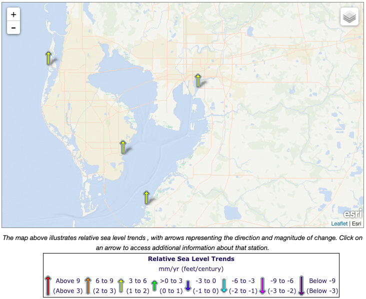
https://tidesandcurrents.noaa.gov/sltrends/
https://api.tidesandcurrents.noaa.gov/mdapi/prod/webapi/stations/id.extension https://api.tidesandcurrents.noaa.gov/mdapi/prod/webapi/stations/8726724.json https://api.tidesandcurrents.noaa.gov/mdapi/prod/webapi/stations/8726724/details.json - “established”: “1973-04-19 00:00:00.0” - “origyear”: “1995-07-27 23:00:00.0” https://api.tidesandcurrents.noaa.gov/mdapi/prod/webapi/stations/8726724/products.json - “name”: “Water Levels”, - “value”: “https://tidesandcurrents.noaa.gov/waterlevels.html?id=8726724”
https://tidesandcurrents.noaa.gov/sltrends/sltrends_station.shtml?id=8726724 https://tidesandcurrents.noaa.gov/sltrends/data/8726724_meantrend.csv
Inundation History - NOAA Tides & Currents
See tbeptools additions:
8726724872667487263848726520coral reefs: ecosystem health, ecotourism
fisheries
energy for hurricanes
background: NOAA Coral Reef Watch Tutorial
Output is stored in a single raster file containing about a little over 13K layers, which seems to read and render reasonably fast (whereas for the more numerous PRISM layers, it was way too slow).
librarian::shelf(
  sf, tbeptools, mapview)

tbshed_buf <- tbshed |>
  st_buffer(10000) |> # buffer by 10 km
  st_bbox() |>
  st_as_sfc() |>
  st_as_sf()

# st_bbox(tbshed_buf) |> round(1)
#  xmin  ymin  xmax  ymax
# -83.0  27.3 -81.8  28.5
# after clipping to non-NA raster values
bbox = c(xmin = -83.0, ymin = 27.2, xmax = -82.3, ymax= 28.5)
sst_bbox <- bbox |>
  sf::st_bbox() |>
  sf::st_as_sfc() |>
  sf::st_as_sf(crs = "+proj=longlat +datum=WGS84 +no_defs")

mapView(tbsegshed, col.regions="gray") +
  mapView(tbshed_buf, col.regions = "blue") +
mapView(sst_bbox, col.regions = "red")librarian::shelf(
marinebon/extractr,
here)
ed_extract(
ed = ed_info("https://coastwatch.noaa.gov/erddap/griddap/noaacrwsstDaily.html"),
var = "analysed_sst",
bbox = c(xmin = -83.0, ymin = 27.2, xmax = -82.3, ymax= 28.5),
aoi = tbeptools::tbsegshed,
zonal_csv = here("data/sst/tbep_sst.csv"),
rast_tif = here("data/sst/tbep_sst.tif"),
mask_tif = F)librarian::shelf(
ggplot2, here, highcharter, lubridate, plotly, readr)
# data("mpg", "diamonds", "economics_long", package = "ggplot2")
# economics_long2 <- dplyr::filter(economics_long, variable %in% c("pop", "uempmed", "unemploy"))
# hchart(economics_long2, "line", hcaes(x = date, y = value01, group = variable))
sst_csv <- here("data/sst/tb_sst.csv")
d_sst <- read_csv(sst_csv, show_col_types = F)
table(d_sst$bay_segment)
# BCB HB LTB MR MTB OTB TCB
# 13169 13169 13169 13169 13169 13169 13169
bay_segment <- "BCB"
d <- d_sst |>
filter(bay_segment == !!bay_segment) |>
mutate(
year = year(time),
# yday = yday(time),
date = sprintf(
"%d-%02d-%02d",
year(today()), month(time), day(time) ) |>
as.POSIXct(),
color = case_when(
year == year(today()) ~ "red",
year == year(today()) - 1 ~ "orange",
.default = "gray") ) |>
# select(year, yday, date, color, val) |>
# arrange(year, yday, date, val)
select(time, year, date, color, val) |>
arrange(year, date, val)
# table(d$yday) |> range()
yrs <- as.character(unique(d$year))
colors <- setNames(rep("darkgray", length(yrs)), yrs)
colors[as.character(year(today()))] <- "red"
colors[as.character(year(today()) - 1)] <- "orange"
librarian::shelf(
slider, scales)
d <- d |>
group_by(year) |>
mutate(
val_sl = slider::slide_mean(
val, before = 3L, after = 3L, step = 1L,
complete = F, na_rm = T),
txt_date = as.Date(time),
txt_val = round(val_sl, 2) ) |>
select(-time) |>
ungroup()
# TODO: darkly theme w/ bslib
g <- ggplot(
d,
aes(
x = date,
y = val_sl,
group = year,
color = factor(year),
date = txt_date,
value = txt_val)) + # frame = yday
geom_line(
# aes(text = text),
alpha = 0.6) +
scale_colour_manual(
values = colors) +
theme(legend.position = "none") +
scale_x_datetime(
labels = date_format("%b %d")) +
labs(
x = "Day of year",
y = "Temperature ºC")
g
# x, y, alpha, color, group, linetype, size
# add color theming
# https://rstudio.github.io/thematic/articles/auto.html
ggplotly(g, tooltip=c("date","value"))
# https://plotly-r.com/scatter-traces 3
# https://plotly-r.com/client-side-linking 16
# https://stackoverflow.com/questions/76435688/how-to-autoplay-a-plotly-chart-in-shiny
d |>
plot_ly(
x = ~date,
y = ~val,
frame = ~yday,
# group = ~year,
# color = ~color,
type = 'scatter',
mode = 'lines',
# marker = list(size = 20),
showlegend = F,
transforms = list(
list(
type = 'groupby',
groups = d$year,
styles = list(
list(target = 2024, value = list(line =list(color = 'red'))),
list(target = 2023, value = list(line =list(color = 'orange'))),
list(target = 2022, value = list(line =list(color = 'darkgray'))) ) ) ) )
animation_button(visible = T) |>
onRender("
function(el,x) {
Plotly.animate(el);
}")
library(plotly)
library(htmlwidgets)
df <- data.frame(
x = c(1,2,1),
y = c(1,2,1),
f = c(1,2,3)
)
df %>%
plot_ly(
x = ~x,
y = ~y,
frame = ~f,
type = 'scatter',
mode = 'markers',
marker = list(size = 20),
showlegend = FALSE
) %>%
animation_button(visible = TRUE) %>%
onRender("
function(el,x) {
Plotly.animate(el);
}")
# https://stackoverflow.com/questions/61152879/change-the-frame-label-in-plotly-animation
DF <- data.frame(
year = rep(seq(1980L, 2020L), each = 12),
month = rep(1:12, 41),
month_char = rep(factor(month.abb), 41),
avg_depth = runif(492) )
# with(DF, paste0(sprintf("%02d", month), " - ", month_char) )
fig <- DF |>
plot_ly(
x = ~year,
y = ~avg_depth,
frame = ~paste0(sprintf("%02d", month), " - ", month_char),
type = 'bar') |>
animation_slider(
currentvalue = list(prefix = "Month: ") )
fig
# https://stackoverflow.com/questions/50843134/r-plotly-animated-chart-only-showing-groups-with-data-in-initial-frame
dates <- 2000:2010
countries <- c("US", "GB", "JP")
df <- merge(dates, countries, all=TRUE)
names(df) <- c("Date", "Country")
df$x <- rnorm(nrow(df))
df$y <- rnorm(nrow(df))
df[1:3, c("x", "y")] <- NA
p <- ggplot(df, aes(x, y, color = Country)) +
geom_point(aes(frame = Date)) + theme_bw()
ggplotly(p)
# other
g <- ggplot(
d,
aes(
x = date,
y = val,
color = factor(year))) +
geom_line(alpha = 0.6) +
scale_colour_manual(
values = colors) +
theme(legend.position = "none")
g
p <- ggplotly(g) |>
onRender("
function(el,x) {
Plotly.animate(el);
}")
p
d |>
hchart(
"line", # "line"
hcaes(
x = date,
y = val,
group = year,
segmentColor = clr),
showInLegend = F)
mpgman2 <- count(mpg, manufacturer, year)
hchart(
mpgman2,
"bar",
hcaes(x = manufacturer, y = n, group = year),
color = c("#7CB5EC", "#F7A35C"),
name = c("Year 1999", "Year 2008"),
showInLegend = c(TRUE, FALSE) # only show the first one in the legend
)Or “Severe Weather”
rnoaa::coops_search()
# swdi - Severe Weather Data Inventory (SWDI) vignetteslr_nc <- here("data/slr/slr_map_txj1j2.nc")
r_slr_gcs <- rast(slr_nc) # 0.5 degree resolution
r_slr_mer <- projectRasterForLeaflet(r_slr_gcs, method="bilinear")
b <- st_bbox(tbsegshed)
r_slr_tb_mer <- rast(slr_nc) |>
crop(b) # |>
# projectRasterForLeaflet(method="bilinear")
# only one value for Tampa Bay extracted at 0.5 degree resolution
# values(r_slr_tb_mer, mat=F, na.rm=T) # 5.368306
b <- st_bbox(tbshed)
plet(r_slr_mer, tiles=providers$Esri.OceanBasemap) |>
addProviderTiles(providers$CartoDB.DarkMatterOnlyLabels) |>
addPolygons(data = tbsegshed) |>
fitBounds(
lng1 = b[["xmin"]], lat1 = b[["ymin"]],
lng2 = b[["xmax"]], lat2 = b[["ymax"]])