Visualise the hydraulic gradient for a bay segment
Usage
util_gw_showgrad(
  pot_rast,
  season = c("dry", "wet"),
  seg,
  segs = tbsubshed,
  shoreline = tbsegdetail,
  buf_segs = NULL
)
Arguments
- pot_rast
SpatRaster(orPackedSpatRaster) of Upper Floridan Aquifer potentiometric head (ft above MSL) as returned byutil_gw_getcontour, or the package datasetscontdry/contwet.- season
character,
"dry"or"wet".- seg
integer, bay segment number (1-7).
- segs
- shoreline
sfobject of bay segment polygons. Defaults totbsegdetail.- buf_segs
named numeric vector of buffer distances (US Survey Feet) in the same format accepted by
util_gw_grad. WhenNULL, season-specific defaults are used (seeutil_gw_gradfor details).
Value
A ggplot object.
Details
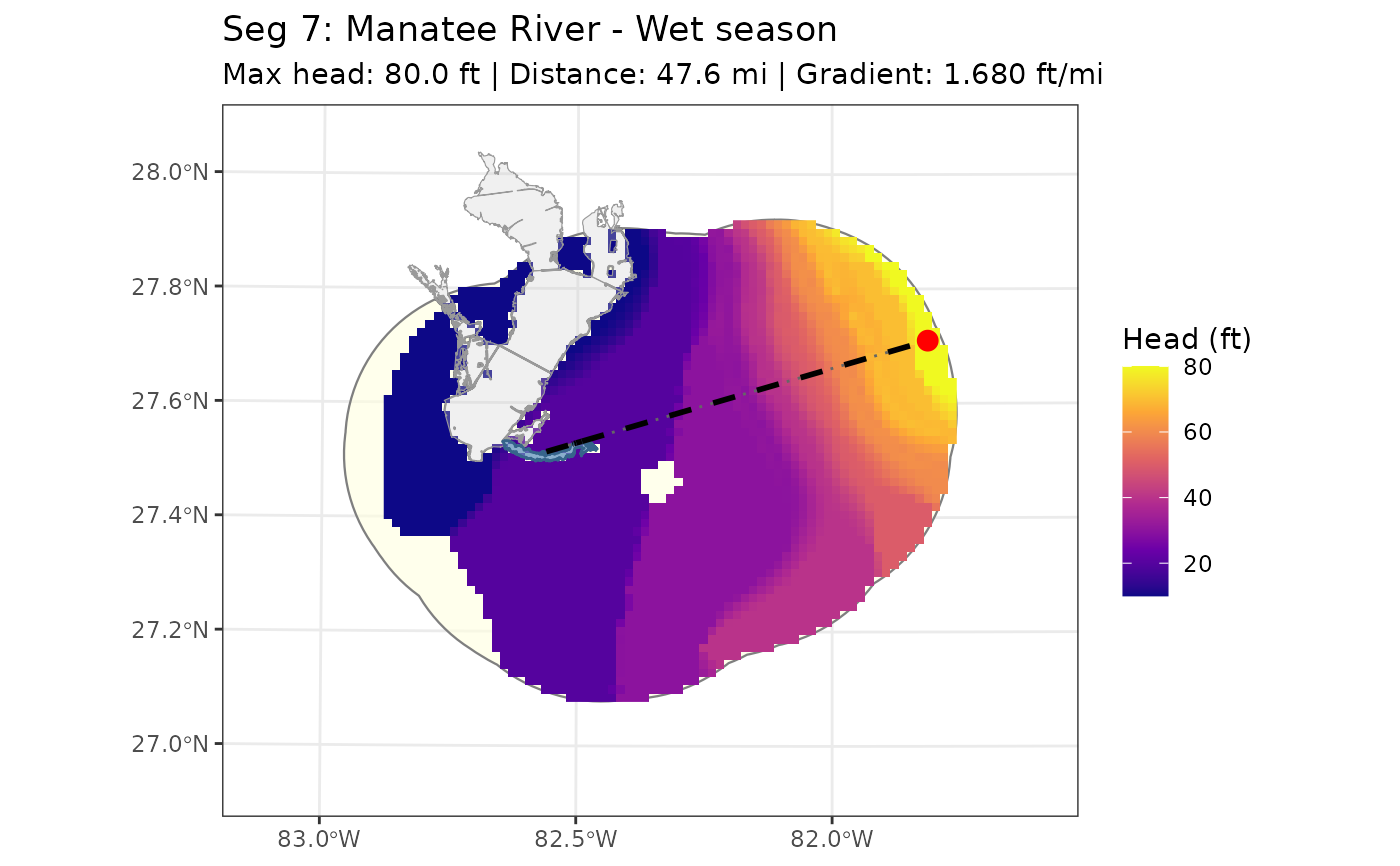
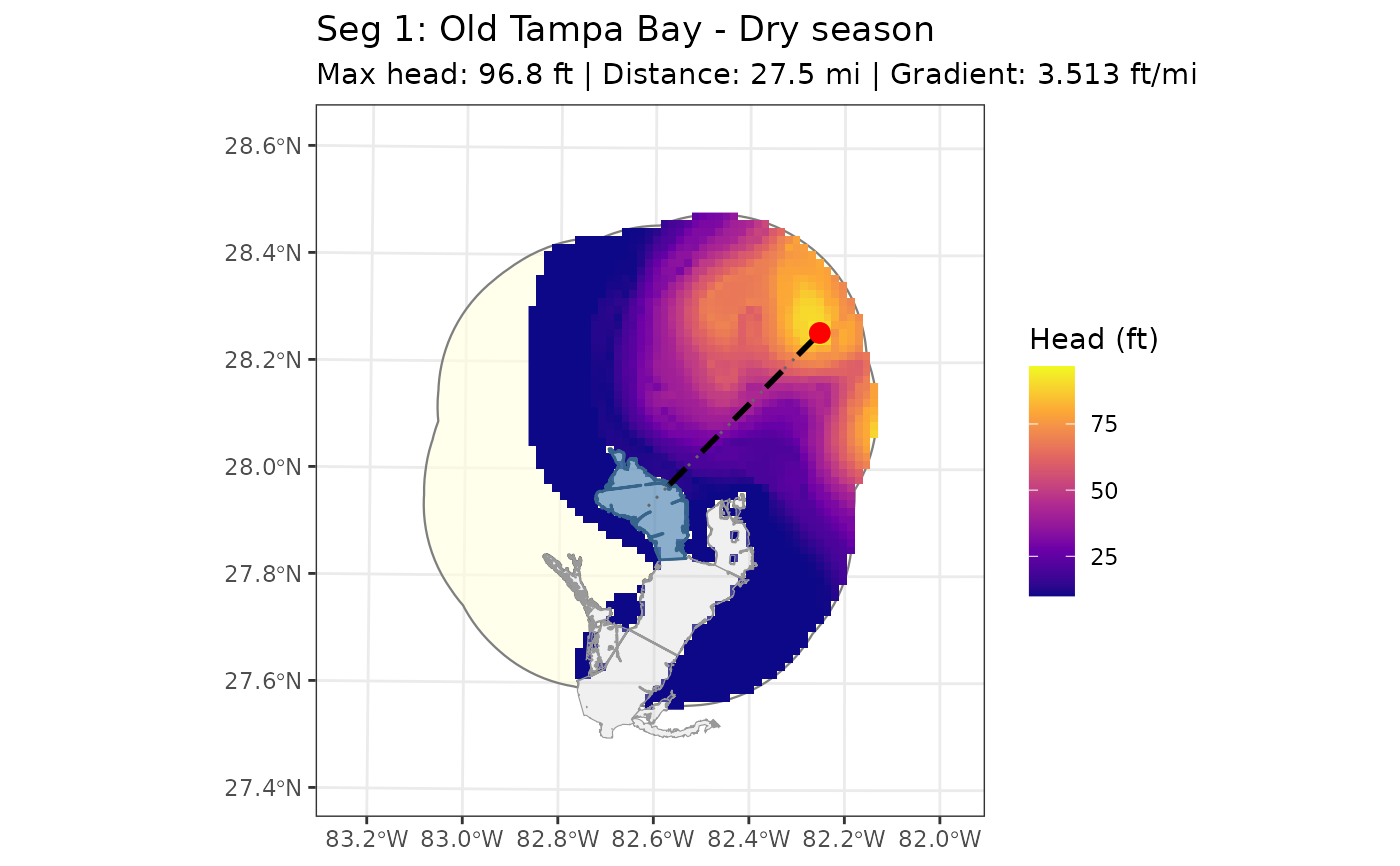
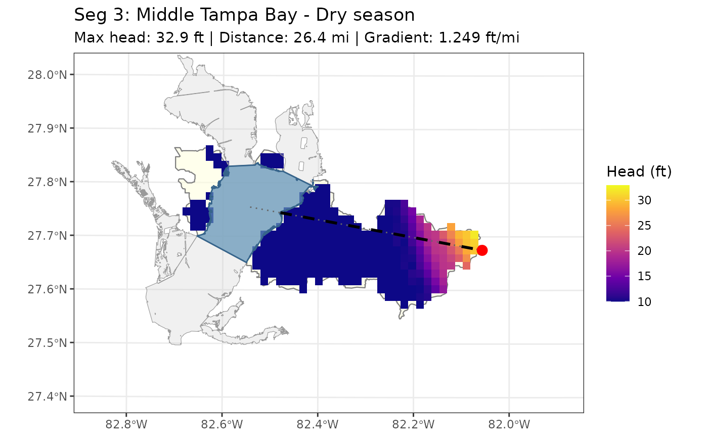
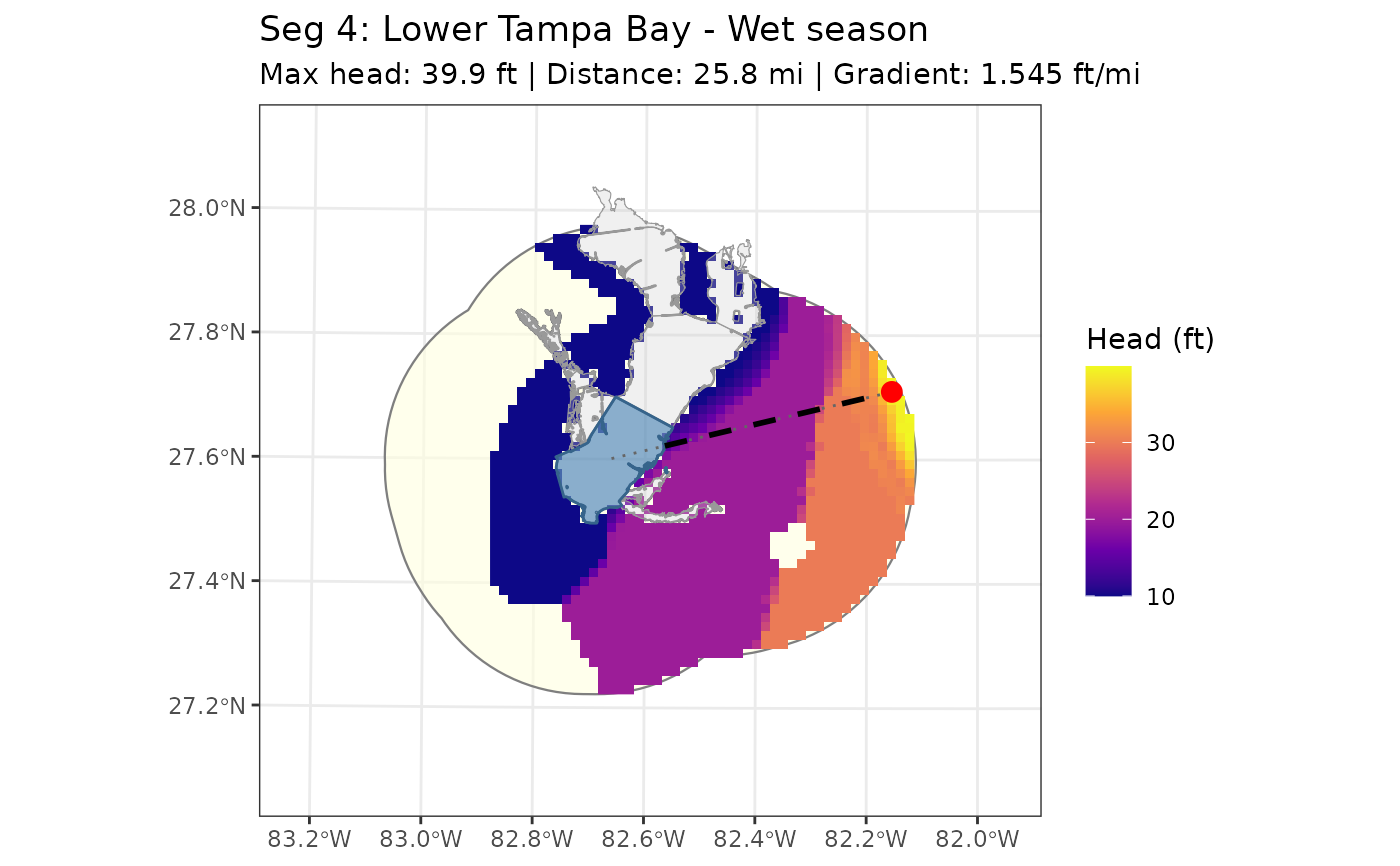
Returns a ggplot2 map for the requested segment showing:
The potentiometric surface (ft) within the search area, coloured by head value.
The search area boundary (light yellow).
All bay segments (grey background) and the target segment (blue).
A dotted line from the bay centroid to the max-head land cell (showing the full transect used in the distance calculation).
A dashed line for the land portion of that transect (the actual gradient distance).
The max-head point (red dot).
The subtitle reports max head (ft), distance (miles), and gradient (ft/mi).
See util_gw_grad for the distance calculation methodology.
Examples
if (FALSE) { # \dontrun{
contdry <- util_gw_getcontour("dry", 2022)
} # }
util_gw_showgrad(contdry, season = "dry", seg = 1)
 util_gw_showgrad(contdry, season = "dry", seg = 3)
#> Warning: Raster pixels are placed at uneven horizontal intervals and will be shifted
#> ℹ Consider using `geom_tile()` instead.
#> Warning: Raster pixels are placed at uneven horizontal intervals and will be shifted
#> ℹ Consider using `geom_tile()` instead.
util_gw_showgrad(contdry, season = "dry", seg = 3)
#> Warning: Raster pixels are placed at uneven horizontal intervals and will be shifted
#> ℹ Consider using `geom_tile()` instead.
#> Warning: Raster pixels are placed at uneven horizontal intervals and will be shifted
#> ℹ Consider using `geom_tile()` instead.
 if (FALSE) { # \dontrun{
contwet <- util_gw_getcontour("wet", 2022)
} # }
util_gw_showgrad(contwet, season = "wet", seg = 4)
if (FALSE) { # \dontrun{
contwet <- util_gw_getcontour("wet", 2022)
} # }
util_gw_showgrad(contwet, season = "wet", seg = 4)
 util_gw_showgrad(contwet, season = "wet", seg = 7)