Groundwater (GW) • tbeploads

library(tbeploads)

Groundwater loads to Tampa Bay are estimated using the three-aquifer framework from Zarbock et al. (1994). The anlz_gw() function computes monthly TN, TP, and hydrologic loads for all bay segments.

Methodology

Three aquifer types contribute to each bay segment each month.

Floridan aquifer: Flow is estimated with Darcy’s Law:

$Q = 7.4805 * 10^{-6} * T * I * L$

where T is transmissivity (ft²/day), I is the hydraulic gradient (ft/mile), and L is the flow zone length (miles). Q is in million gallons per day (MGD). Transmissivity and flow zone length are fixed constants per segment from Zarbock et al. (1994). Hydraulic gradients are season-specific: months 1-6 and 11-12 are dry season; months 7-10 are wet season. The util_gw_grad() function computes gradients from FDEP potentiometric surface contours for the dry and wet seasons (see below).

Monthly nutrient loads (kg/month) are:

$Load = Q * C * 8.342 * 30.5 / 2.2$

where C is the TN or TP concentration in mg/L.

Monthly hydrologic load (m³/month) is:

$Load = Q * 3785 * 30.5$

Surficial and intermediate aquifers: Loads are fixed monthly constants per segment derived from 1995-1998 (surficial) and 1999-2003 (intermediate) SWFWMD monitoring data. These values have not changed since the original analysis.

Hydraulic gradient computation

Hydraulic gradients are computed from FDEP Upper Floridan Aquifer potentiometric surface contour lines using util_gw_getcontour() and util_gw_grad().

Downloading and rasterizing contours

util_gw_getcontour() downloads biannual FDEP contour lines (May = dry, September = wet) from the Florida Geological Survey ArcGIS REST service. Rather than working directly with the vector contour lines, the function rasterizes them to a 1-mile grid using inverse distance weighting (IDW, 5-mile radius) followed by iterative focal gap-filling. The spatial extent of the download covers the Tampa Bay watershed (tbfullshed) buffered outward by 40 miles to capture high potentiometric values outside of the surficial subwatersheds that drive groundwater flow. The IDW radius was deliberately set to 5 miles (rather than the contour spacing) to prevent extrapolation into data-sparse coastal and northern areas.

contdry <- util_gw_getcontour("dry", 2022)
contwet <- util_gw_getcontour("wet", 2022)

The package datasets contdry and contwet contain pre-computed 2022 rasters stored as PackedSpatRaster objects. Unwrap them with terra::unwrap() before use or pass them directly to util_gw_grad() and util_gw_showgrad(), which unwrap automatically.

Computing gradients

util_gw_grad() finds the maximum potentiometric head within each segment’s search area, then measures the distance from the shoreline to that high point using a centroid-based transect:

A line is drawn from the bay segment centroid to the max-head land cell.
The portion of that line inside the bay polygon (from centroid to shoreline crossing) is subtracted from the total length.
The remaining land-side distance is used as the gradient base.

This approach avoids measuring to an extreme geographic corner of the shoreline (e.g., the northeast tip of Middle Tampa Bay), giving a more representative transect.

Search areas to find the maximum head for each segment are controlled by the buf_segs parameter, which buffers the subwatershed polygon outward and removes bay water. Default buffer distances (calibrated against 2021 SAS reference values) are applied automatically:

Dry season: Old Tampa Bay (seg 1) buffered ~19 miles to capture the potentiometric high north/northeast of the standard watershed boundary.
Wet season: same as dry, plus Lower Tampa Bay (4), Terra Ceia Bay (6), and Manatee River (7) each buffered ~19 miles to unlock wet-season dynamic computation.

Zero-gradient segments (hardcoded, not computed dynamically) reflect deliberate decisions from prior loading analyses (Zarbock et al. 1994):

Boca Ciega Bay (segments 5 and 55), both seasons: the heavily urbanized coastal watershed has no meaningful Floridan Aquifer recharge directed toward the bay.
Lower Tampa Bay (4), Terra Ceia Bay (6), Manatee River (7), dry season only: the potentiometric gradient is negligible during the dry season.

Hillsborough Bay (segment 2) uses a three-zone weighted average (Polk County 0.4, Pasco County 0.3, Alafia River 0.3) following the original flow net analysis in the SAS code.

Benchmark warning: util_gw_grad() compares computed gradients against 2021 SAS reference values and issues a warning for any non-zero segment that deviates by more than 50%, making it easy to detect anomalous potentiometric surfaces when running future years.

util_gw_grad(contdry, season = "dry")
#>   bay_seg     grad
#> 1       1 3.513075
#> 2       2 2.790798
#> 3       3 1.249106
#> 4       4 0.000000
#> 5       5 0.000000
#> 6       6 0.000000
#> 7       7 0.000000
#> 8      55 0.000000
util_gw_grad(contwet, season = "wet")
#>   bay_seg     grad
#> 1       1 4.021441
#> 2       2 3.319684
#> 3       3 2.006550
#> 4       4 1.544803
#> 5       5 0.000000
#> 6       6 1.386061
#> 7       7 1.679699
#> 8      55 0.000000

Visualising gradients

util_gw_showgrad() produces a map for a single segment showing the potentiometric surface within the search area, the centroid-to-head transect, and the computed gradient.

util_gw_showgrad(contdry, season = "dry", seg = 1)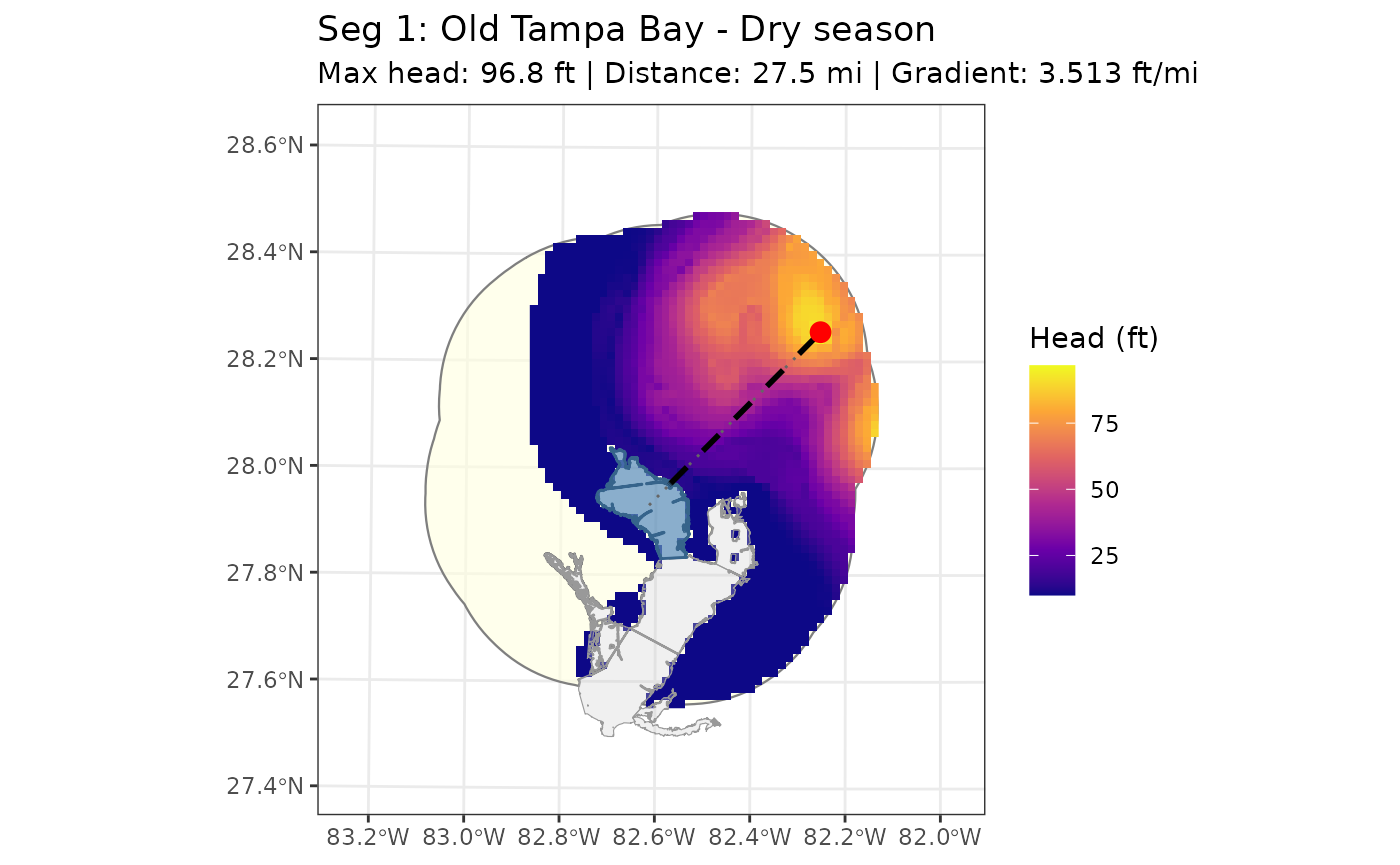

util_gw_showgrad(contwet, season = "wet", seg = 7)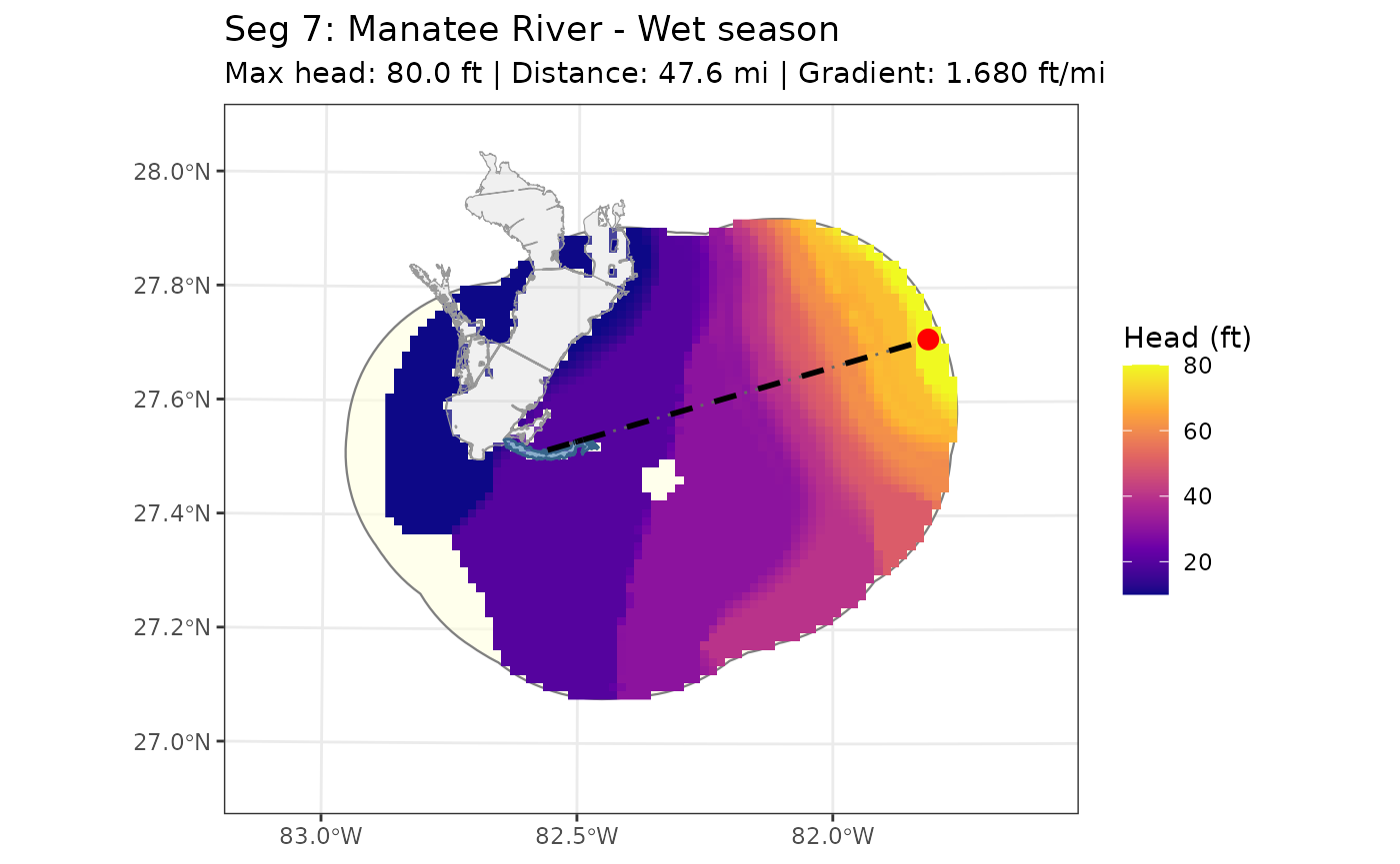

Floridan aquifer concentrations

Floridan aquifer TN and TP concentrations (mg/L) can be obtained from the Water Atlas API using util_gw_getwq(). The default stations are 18340 (CR 581 North Fldn) and 18965 (SR 52 and CR 581 Deep), the two Pasco County Floridan aquifer monitoring wells used in the 2022-2024 loading analysis. Old Tampa Bay uses the first station mean only and Hillsborough Bay uses the arithmetic mean of both station means. The rest of the bay segments retain fixed historical values from the 1995-1998 SWFWMD analysis used in every loading cycle through 2021.

wqdat <- util_gw_getwq()

When wqdat = NULL (the default in anlz_gw()), hardcoded concentrations from the 2022-2024 analysis are used directly.

Estimating groundwater loads

anlz_gw() takes potentiometric surface rasters for the dry and wet seasons as required inputs, along with a year range. Gradients are computed once from the supplied rasters via util_gw_grad() and applied to every year in the range.

The package datasets contdry and contwet are pre-computed 2022 rasters stored as PackedSpatRaster objects and can be passed directly:

gw <- anlz_gw(contdry, contwet, yrrng = c(2022, 2024))
head(gw)
#>   Year Month source        segment      tn_load     tp_load   hy_load
#> 1 2022     1     GW Boca Ciega Bay 0.0004188783 0.003957298 0.0132126
#> 2 2022     2     GW Boca Ciega Bay 0.0004188783 0.003957298 0.0132126
#> 3 2022     3     GW Boca Ciega Bay 0.0004188783 0.003957298 0.0132126
#> 4 2022     4     GW Boca Ciega Bay 0.0004188783 0.003957298 0.0132126
#> 5 2022     5     GW Boca Ciega Bay 0.0004188783 0.003957298 0.0132126
#> 6 2022     6     GW Boca Ciega Bay 0.0004188783 0.003957298 0.0132126

Load columns are in tons/month and hy_load is in million m³/month.

To run the analysis for a new year, first download updated potentiometric surfaces from FDEP, then pass them to anlz_gw():

contdry <- util_gw_getcontour("dry", 2025)
contwet <- util_gw_getcontour("wet", 2025)
gw <- anlz_gw(contdry, contwet, yrrng = c(2025, 2025))

To pass concentrations retrieved from the Water Atlas API:

wqdat  <- util_gw_getwq()
gw_api <- anlz_gw(contdry, contwet, yrrng = c(2022, 2024), wqdat = wqdat)

Temporal summary

Setting summtime = 'year' sums monthly loads to annual totals.

anlz_gw(contdry, contwet, yrrng = c(2022, 2024), summtime = 'year')

References

Zarbock, H., A. Janicki, D. Wade, D. Heimbuch, and H. Wilson. 1994. Estimates of Total Nitrogen, Total Phosphorus, and Total Suspended Solids Loadings to Tampa Bay, Florida. Nos. 04-94. Tampa Bay National Estuary Program.