3  Open science for impactful products

3.1 Goals and motivation

This is the third module in our workshop on open science. Now we focus on how Quarto can be used as a document preparation system to generate easily shared web content.

• Goal: understand best practices for reproducible documents using Quarto
• Motivation: cultivate your analyses as living, shared resources

3.2 Quarto

Quarto is a relatively new document preparation system that lets you create reproducible and dynamic content that is easily shared with others. Quarto is integrated with RStudio and allows you to combine plain text language with analysis code in the same document.

Quarto belongs to a class of literate programming tools called dynamic documents (Knuth 1984). It is not the first of its kind, but it builds substantially on its predecessors by bridging multiple programming langues.

Advantages of creating analyses using Quarto include:

1. Clear demonstration of a workflow using plain text and code
2. Reproducible materials allow others to use your work
3. Easily shared content (e.g., on GitHub)
4. Keeping the data, analysis, and writing all in the same place

This next section will run through the very basics of creating a Quarto document, some of the options for formatting, and how to generate shared content. You’ll follow along in this module.

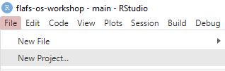
1. Create a new project in RStudio, first open RStudio and select “New project” from the File menu at the top.

   

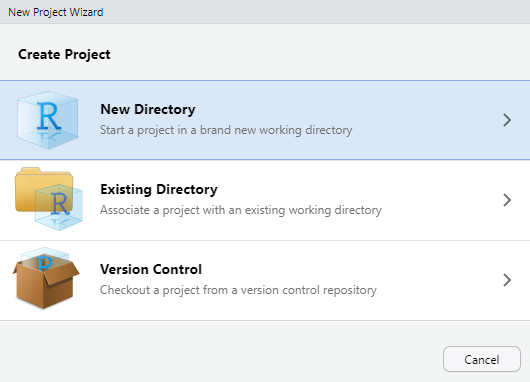
   Then select “New Directory”. Create a directory in a location that’s easy to find.

   

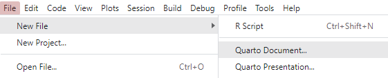
2. Open a new Quarto file from the File menu under New file > Quarto Document.

   

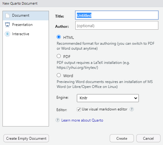
   Enter a title for the document (e.g., “Quarto practice”) and your name as the author. Use the defaults for the other options and hit “Create”.

   

   Save the file in the project root directory (give it any name you want).

3. Let’s get familiar with the components of a Quarto document.

   Tip

   The three main components of a Quarto document are:

   • YAML
   • Code chunks
   • Plain or Markdown text

   The new file includes some template material showing the main components of a Quarto document. The content at the top is called YAML, which defines global options for the document.

   ---
   title: "Quarto practice"
   author: "Marcus Beck"
   editor: visual
   ---

   You’ll also notice that there’s a button on the top-left that lets you toggle between “source” or “visual” editor mode. The source editor simply lets you add text to the document, whereas the visual editor lets you add content that is partially rendered. First time Quarto users may prefer the visual editor.

   

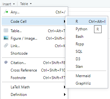
   Using the visual editor, we can insert a code chunk (or code cell). This can be done by selecting the appropriate option from the Insert menu. Note the variety of programming langues that can be used with the code chunk.

   

   We can enter any code we want in the code chunks, including options for how the code chunk is evaluated. Options are specified using the hashpipe notation, #|.

   ```{r}
   #| echo: true
   print('Hello Quarto!')
   ```

   When the file is rendered, the code is run and results displayed in the output. There are many options to change how code chunks are executed, which we’ll discuss below.

   print('Hello Quarto!')

   [1] "Hello Quarto!"

   We can also run the code chunks separately without rendering the file using the arrow buttons on the top right in the source document. This can be useful for quickly evaluating your code as you include it in the file.

   Tip

   Code chunks are executed in the order they appear in the document when a .qmd file is rendered.

   Descriptive text can be entered anywhere else in the file. This is where we can describe in plain language what our analysis does or any other relevant information. Text can be entered as-is or using simple markdown text that can format the appearance of the output. If you’re using the visual editor, you can use some of the items in the file menu to modify the text appearance. In the source editor, you can manually enter markdown text:

   
   I  can write anything I want right here. Here's some **bold text**.
   
   I can also make lists
   
   1. Item 1
   1. Item 2
   
   

   When the file is rendered, the markdown text will be formatted. The text will already be formatted if you’re using the visual editor:

   I can write anything I want right here. Here’s some bold text.

   I can also make lists

   1. Item 1
   2. Item 2

4. Render the .qmd file to the output format.

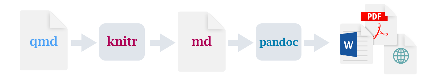
   The source file is a .qmd document. We need to render the document to create the output format - HTML (default), PDF, or Word. The following happens when you hit the render button at the top.

   

   Here’s what your RStudio session should look like (note the three parts of the source .qmd document - YAML, code chunk, and Markdown text). The rendered HTML file will appear in the Viewer pane on the right.

   

   Tip

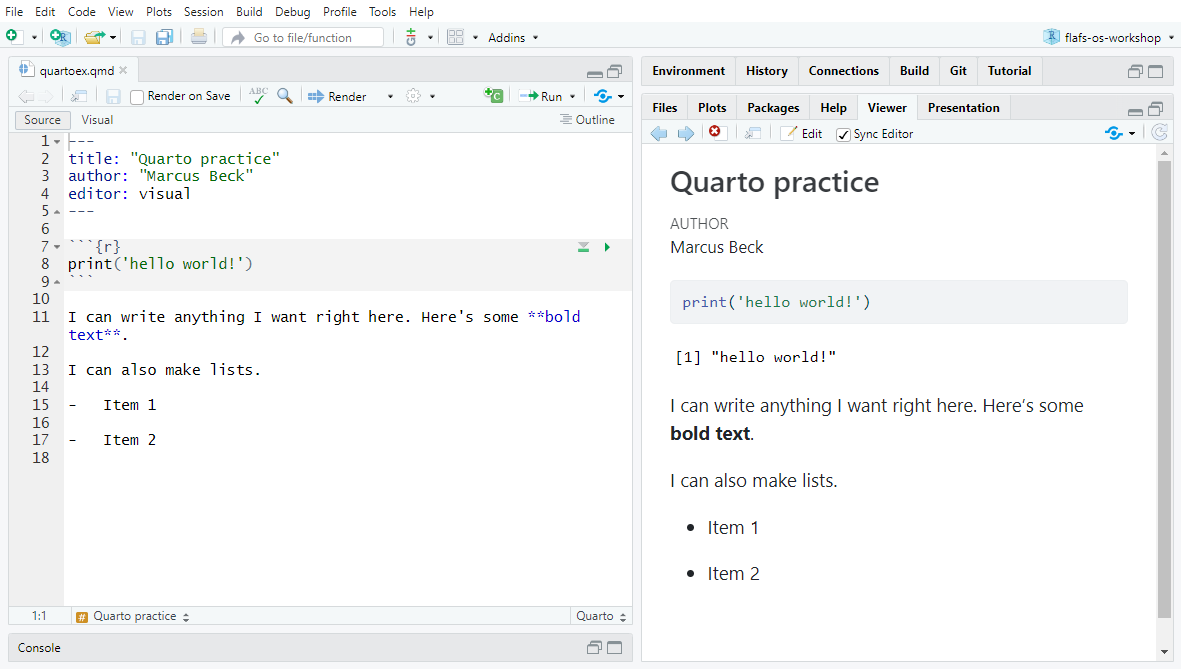
   A rendered Quarto document as an HTML, PDF, Word, or other file format is stand-alone and can be shared with anybody!

3.2.1 Code chunk options

The behavior of the code chunks when the file is rendered can be changed using the many options available in Quarto. This can be useful for a few reasons.

1. Only displaying the output of a code chunk
2. Only displaying the code and not running the chunk
3. Running the code without displaying output for use in other parts of the document
4. Suppressing warnings and messages
5. Defining table or figure options (e.g., height, width, captions, etc.)

Code chunk options can be applied globally to all chunks in the document or separately for each chunk.

To apply them globally, they’ll look something like this in the YAML, where options are added after execute:

---
title: "My Document"

execute: 
  echo: false
  warning: false
---

Tip

Be careful with indentation in the YAML, the document won’t render if the indentation is incorrect.

To apply to individual code chunks, use the #| (hashpipe) notation at the top of the code chunk. This will override any global options if you’ve included them in the top YAML. Below, echo: true indicates that the code will be displayed in the rendered output.

```{r}
#| echo: true
plot(1:10)
```

Here’s a short list of other useful execution options:

Option	Description
eval	Evaluate the code chunk (if false, just echos the code into the output).
echo	Include the source code in output
output	Include the results of executing the code in the output (true, false, or asis to indicate that the output is raw markdown and should not have any of Quarto’s standard enclosing markdown).
warning	Include warnings in the output.
error	Include errors in the output (note that this implies that errors executing code will not halt processing of the document).
include	Catch all for preventing any output (code or results) from being included (e.g. include: false suppresses all output from the code block).
message	Include messages in rendered output

R code can also be executed “inline” outside of code chunks. This can be useful if you want to include statements that reference particular values or information that is linked directly to data. Inline R code is entered using the r syntax.

I can enter inline text like `r 1 + 1`.

Text with inline R code will look like this when the document is rendered.

I can enter inline text like 2.

3.2.2 Figures and tables

Figures and tables are easily added in Quarto, using either R code or importing from an external source.

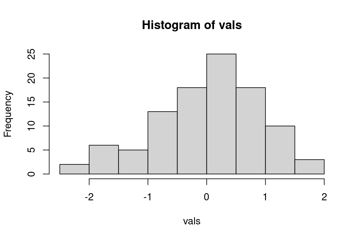
Any figures created in code chunks will be included in the rendered output. Relevant code chunk options for figures include fig-height, fig-width, fig-cap, label (for cross-referencing) and fig-align.

```{r}
#| label: fig-myhist
#| fig-height: 4
#| fig-width: 6
#| fig-cap: "Here's my awesome histogram."
#| fig-align: "center"
vals <- rnorm(100)
hist(vals)
```

Figure 3.1: Here’s my awesome histogram.

Figures can be cross-referenced in the text using the @ notation with the figure label.

Here's a cross-reference to @fig-myhist.

When the file is rendered, the appropriate figure number will be displayed with a link to the figure:

Here’s a cross-reference to Figure 3.1.

Similarly, tabular output can be created inside code chunks.

```{r}
#| label: tbl-mytable
#| tbl-cap: "Here's my awesome table."
totab <- data.frame(
  Species = c('Bluegill', 'Largemouth bass', 'Crappie'),
  Count = c(12, 5, 4)
)
knitr::kable(totab)
```

Table 3.1: Here’s my awesome table.

Species	Count
Bluegill	12
Largemouth bass	5
Crappie	4

And a cross-reference:

Here's a cross-reference to @tbl-mytable.

Here’s a cross-reference to Table 3.1.

Tip

Label tags for tables and figures should include the tbl- or fig- prefix for proper cross-referencing.

Figures can also be imported from an external source (e.g., from your computer or the web) using the ![]() notation, where the image is in the img folder in my working directory. You can also simply add a figure from the file menu using the Visual editor.

![](img/blackcrappie.jpg)

You can also add a figure from a URL using the same notation.

![](https://www.bigcatchflorida.com/media/1174/blackcrappie.jpg)

Adding captions and labels to external figures looks something like this:

![Here's a beautiful crappie](img/blackcrappie.jpg){#fig-crappie}

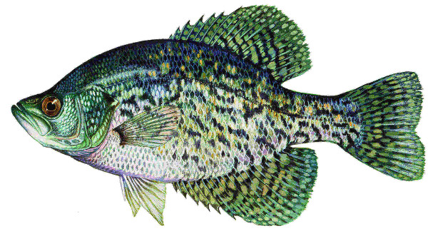
Figure 3.2: Here’s a beautiful crappie

The cross-reference is done the same.

Here's a cross-reference to @fig-crappie

Here’s a cross-reference to Figure 3.2.

Likewise, tables can be imported from an external source (e.g., Excel). You’ll want to do this in a code chunk and add the appropriate options (e.g., to cross-reference Table 3.2).

```{r}
#| label: tbl-habitats
#| tbl-cap: "The first six rows of our tidy data"
mytab <- readxl::read_excel('data/tidy.xlsx')[1:6, ]
knitr::kable(mytab)
```

Table 3.2: The first six rows of our tidy data

Location	Habitat	Year	Acres	Category
Clear Bay	Seagrass	2019	519	B
Clear Bay	Oysters	2019	390	B
Clear Bay	Sand	2019	742	C
Fish Bay	Seagrass	2019	930	B
Fish Bay	Oysters	2019	680	A
Fish Bay	Sand	2019	611	A

Visit these links for full details on figures and tables in Quarto. R also has a rich library of packages for producing tables, most of which play nice with Quarto.

3.2.3 Output options

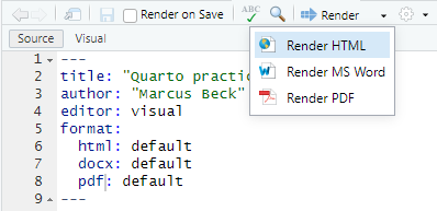
Rendering a Quarto file to an HTML, PDF, or Word document is as simple as adding the appropriate option to the YAML. This is done by choosing the format when you create a new Quarto file:

The output format can also be added in the YAML of the document.

---
title: "Quarto practice"
author: "Marcus Beck"
editor: visual
format: html
---

Tip

The default output format is HTML and it does not need to be added explicitly to the YAML.

Alternative formats are specified the same way (i.e., Word and PDF).

---
title: "Quarto practice"
author: "Marcus Beck"
editor: visual
format: docx
---

---
title: "Quarto practice"
author: "Marcus Beck"
editor: visual
format: pdf
---

You can also specify multiple formats (note the indentation). The default setting just indicates that we want to use all default options for each format and this option must be included.

---
title: "Quarto practice"
author: "Marcus Beck"
editor: visual
format: 
  html: default
  docx: default
  pdf: default
---

You can use the dropdown menu to render each file format one at a time. The dropdown menu will show the options that are included in the YAML.

You can also render all formats at once using the quarto package in the console. The path to your file will differ depending on where it is in your working directory.

quarto::quarto_render('data/quartoex.qmd')

Or you can render all formats at once using the render command in the terminal (terminal tab, bottom left pane of RStudio). This requires the separate installation of Quarto described in the setup. This is the Quarto Command Line Interface (CLI).

Terminal

quarto render data/quartoex.qmd

Rendering a file to PDF uses LaTeX and you’ll need to install tinytex before you can use this option. This can also be done in the terminal.

Terminal

quarto install tool tinytex

There are several options you can include in the YAML to control the formatting of the output. Some of the options apply to all format types, whereas others are specific to a type. Here’s an example building out these options.

---
title: "Quarto practice"
author: "Marcus Beck"
editor: visual
toc: true 
number-sections: true
format: 
  html: 
    code-fold: true
  docx: default
  pdf: 
    geometry: 
      - top=30mm
      - left=0mm
---

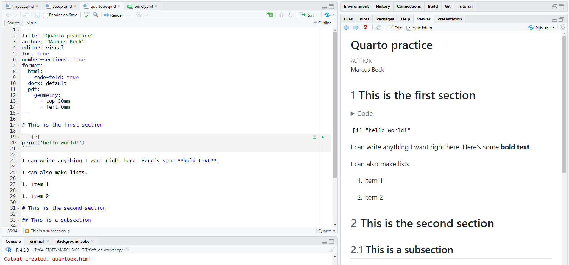
In the above example, there are two new options that apply globally to the HTML, Word, and PDF outputs. Specifically, we’ve indicated that we’d like a table of contents (toc: true) and that the sections should be numbered (number-sections: true) in the rendered documents.

We’ve also added some specific options to the HTML and PDF output. For the HTML output, we’ve indicated that we want the code chunks to be folded (i.e., toggle between seen and not seen, code-fold: true). For the PDF output, we’ve changed the geometry of the margins using the geometry options.

Here’s what the HTML output would look like:

There are many other options available for each output format, as well as other format types. View the full list here.

3.2.4 Citations and References

One of the more valuable aspects of Quarto is the ability to easily add and reference other works in your document. This includes finding papers and reports, citing them in your document, and formatting references - all with relative ease in Quarto.

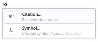
You can of course do this using the source editor, but it’s slightly easier using the visual editor. If we switch to visual mode (top-left button of the .qmd file), you can type a forward-slash to view a menu of items to insert in the document. Just start typing text to search items to insert.

Tip

The Insert Anything tool in the visual editor is useful to… insert anything! Just execute / at the beginning of a line or Ctrl/Cmd + / after some text.

You can also insert a citation from the menu at the top of the .qmd file.

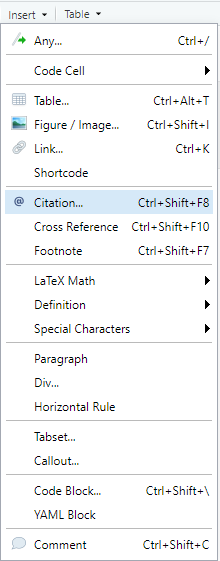
Either option will open the citation menu where you can add citations from a variety of sources (ie., Zotero, DOI, CrossRef, PubMed, or DataCite).

For example, we can copy/paste a DOI to find a reference of interest.

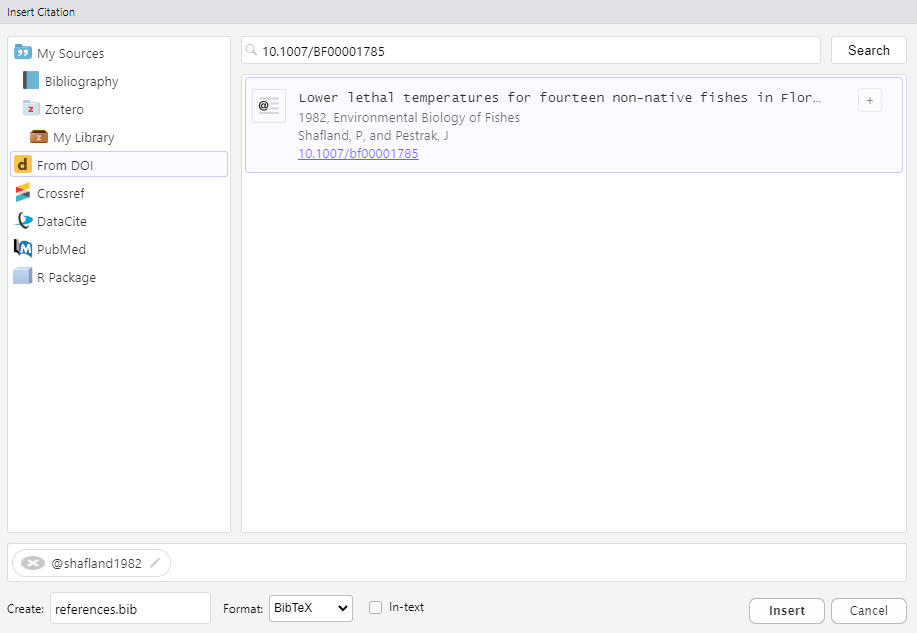
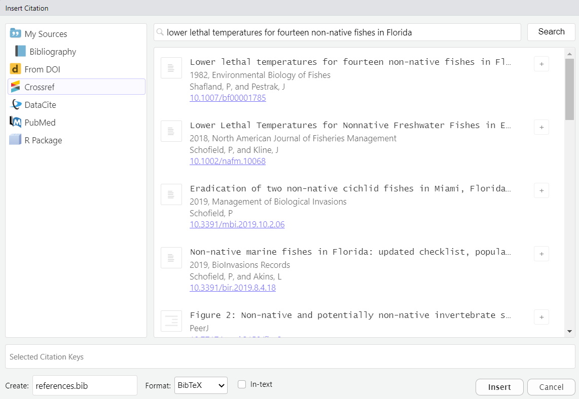
Or we can search by title.

Once the paper is found, you can click the Insert button to add it to your document. This adds a reference file, information in the YAML, and the in-text citation. The reference file will be called references.bib by default and includes a BibTeX formatted reference that looks like this:

@article{shafland1982,
    title = {Lower lethal temperatures for fourteen non-native fishes in Florida},
    author = {Shafland, Paul L. and Pestrak, James M.},
    year = {1982},
    month = {03},
    date = {1982-03},
    journal = {Environmental Biology of Fishes},
    pages = {149--156},
    volume = {7},
    number = {2},
    doi = {10.1007/bf00001785},
    url = {http://dx.doi.org/10.1007/BF00001785},
    langid = {en}
}

The YAML file will now indicate the reference file to use that includes the references (bibliography: references.bib).

---
title: "Quarto practice"
author: "Marcus Beck"
editor: visual
bibliography: references.bib
toc: true 
number-sections: true
format: 
  html: 
    code-fold: true
  docx: default
  pdf: 
    geometry: 
      - top=30mm
      - left=0mm
---

The text citation will look like this, where @ is the tag used to reference the citation using the identifier from the references file.

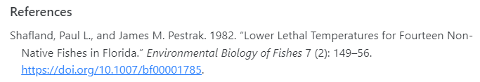
Many non-native species in Florida have lower lethal temperatures [@shafland1982].

When the Quarto file is rendered, the citation will be formatted and you’ll see it added to the references section at the end of the document.

Many non-native species in Florida have lower lethal temperatures (Shafland and Pestrak 1982).

The @ citation syntax also has different options for displaying the citation in the text (full explanation here). For example, omitting the brackets does the following:

@shafland1982 state that many non-native species in Florida have lower lethal temperatures.

Shafland and Pestrak (1982) state that many non-native species in Florida have lower lethal temperatures.

Additional information about citations in Quarto can be found here.

3.2.5 Publishing

A rendered Quarto file can be shared with anyone as a standalone document. The file can also be hosted online and shared by URL. This latter approach is useful to make the document available to anyone with the web address.

The easiest way to do this is to publish your document to RPubs, a free service from Posit for sharing web documents. Click the publish button on the top-right of the editor toolbar. You will be prompted to create an account if you don’t have one already.

This can also be done using the quarto R package in the console.

quarto::quarto_publish_doc(
  "data/quartoex.qmd", 
  server = "rpubs.com"
  )

You can also use the Quarto CLI in the terminal. Here we are publishing the document to Quarto Pub.

Terminal

quarto publish quarto-pub data/quartoex.qmd

If your Quarto document is in an RStudio project on GitHub, you can also publish to GitHub Pages.

Terminal

quarto publish gh-pages data/quartoex.qmd

3.3 Summary

In this module we learned the basics of creating dynamic documents with Quarto that combine markdown text with R code. There’s much, much more Quarto can do for you. Please visit https://quarto.org/ for more information on how you can use these documents to fully leverage their potential for open science.

Knuth, Donald Ervin. 1984. “Literate Programming.” The Computer Journal 27 (2): 97–111. https://doi.org/10.1093/comjnl/27.2.97.

Shafland, Paul L., and James M. Pestrak. 1982. “Lower Lethal Temperatures for Fourteen Non-Native Fishes in Florida.” Environmental Biology of Fishes 7 (2): 149–56. https://doi.org/10.1007/bf00001785.