2  Dynamic: Quarto docs

Learning Objectives

Use the Quarto document preparation system to create dynamic documents that combine text and code. Learn how to share these documents with colleagues.

2.1 Install quarto

Ensure you have the quarto R package installed. Look in RStudio’s Packages pane and install if not found when searching for “quarto”.

Additionally, you can install the Quarto Command Line Interface (CLI). This will allow you to run Quarto from the command line and includes additional features not included with the R package. See the quarto setup section for more info.

2.2 Quarto overview

Quarto is a relatively new document preparation system that lets you create reproducible and dynamic content that is easily shared with others. Quarto is integrated with RStudio and allows you to combine plain text language with analysis code in the same document.

Quarto belongs to a class of literate programming tools called dynamic documents (Knuth 1984). It is not the first of its kind, but it builds substantially on its predecessors by bridging multiple programming langues.

Advantages of creating analyses using Quarto include:

1. Clear demonstration of a workflow using plain text and code
2. Reproducible materials allow others to use your work
3. Easily shared content (e.g., on GitHub)
4. Keeping the data, analysis, and writing all in the same place

This next section will run through the very basics of creating a Quarto document, some of the options for formatting, and how to generate shared content. You’ll follow along in this module.

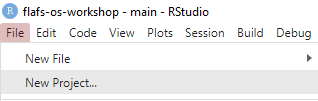
1. Create a new project in RStudio, first open RStudio and select “New project” from the File menu at the top.

   

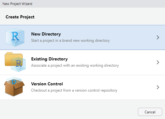
   Then select “New Directory”. Create a directory in a location that’s easy to find.

   

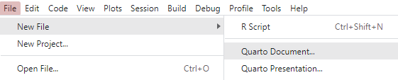
2. Open a new Quarto file from the File menu under New file > Quarto Document.

   

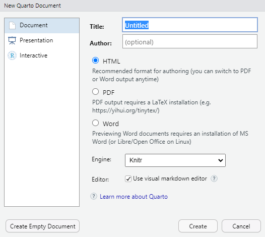
   Enter a title for the document (e.g., “Quarto practice”) and your name as the author. Use the defaults for the other options and hit “Create”.

   

   Save the file in the project root directory (give it any name you want).

3. Let’s get familiar with the components of a Quarto document.

   Tip

   The three main components of a Quarto document are:

   • YAML
   • Code chunks
   • Plain or Markdown text

   The new file includes some template material showing the main components of a Quarto document. The content at the top is called YAML, which defines global options for the document.

   ---
   title: "Quarto practice"
   author: "Marcus Beck"
   editor: visual
   ---

   You’ll also notice that there’s a button on the top-left that lets you toggle between “source” or “visual” editor mode. The source editor simply lets you add text to the document, whereas the visual editor lets you add content that is partially rendered. First time Quarto users may prefer the visual editor.

   

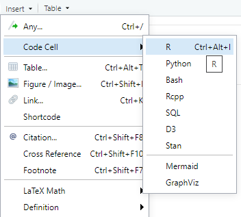
   Using the visual editor, we can insert a code chunk (or code cell). This can be done by selecting the appropriate option from the Insert menu. Note the variety of programming langues that can be used with the code chunk.

   

   We can enter any code we want in the code chunks, including options for how the code chunk is evaluated. Options are specified using the hashpipe notation, #|.

   ```{r}
   #| echo: true
   print('Hello Quarto!')
   ```

   When the file is rendered, the code is run and results displayed in the output. There are many options to change how code chunks are executed, which we’ll discuss below.

   print('Hello Quarto!')

   [1] "Hello Quarto!"

   We can also run the code chunks separately without rendering the file using the arrow buttons on the top right in the source document. This can be useful for quickly evaluating your code as you include it in the file.

   Tip

   Code chunks are executed in the order they appear in the document when a .qmd file is rendered.

   Descriptive text can be entered anywhere else in the file. This is where we can describe in plain language what our analysis does or any other relevant information. Text can be entered as-is or using simple markdown text that can format the appearance of the output. If you’re using the visual editor, you can use some of the items in the file menu to modify the text appearance. In the source editor, you can manually enter markdown text:

   
   I  can write anything I want right here. Here's some **bold text**.
   
   I can also make lists
   
   1. Item 1
   1. Item 2
   
   

   When the file is rendered, the markdown text will be formatted. The text will already be formatted if you’re using the visual editor:

   I can write anything I want right here. Here’s some bold text.

   I can also make lists

   1. Item 1
   2. Item 2

4. Render the .qmd file to the output format.

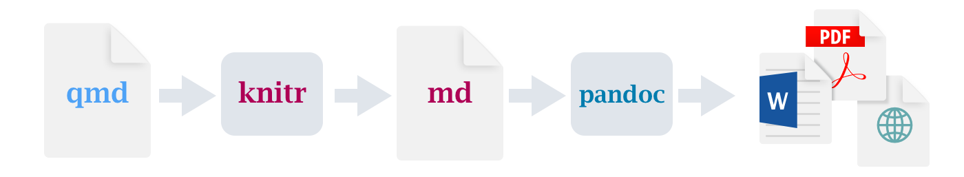
   The source file is a .qmd document. We need to render the document to create the output format - HTML (default), PDF, or Word. The following happens when you hit the render button at the top.

   

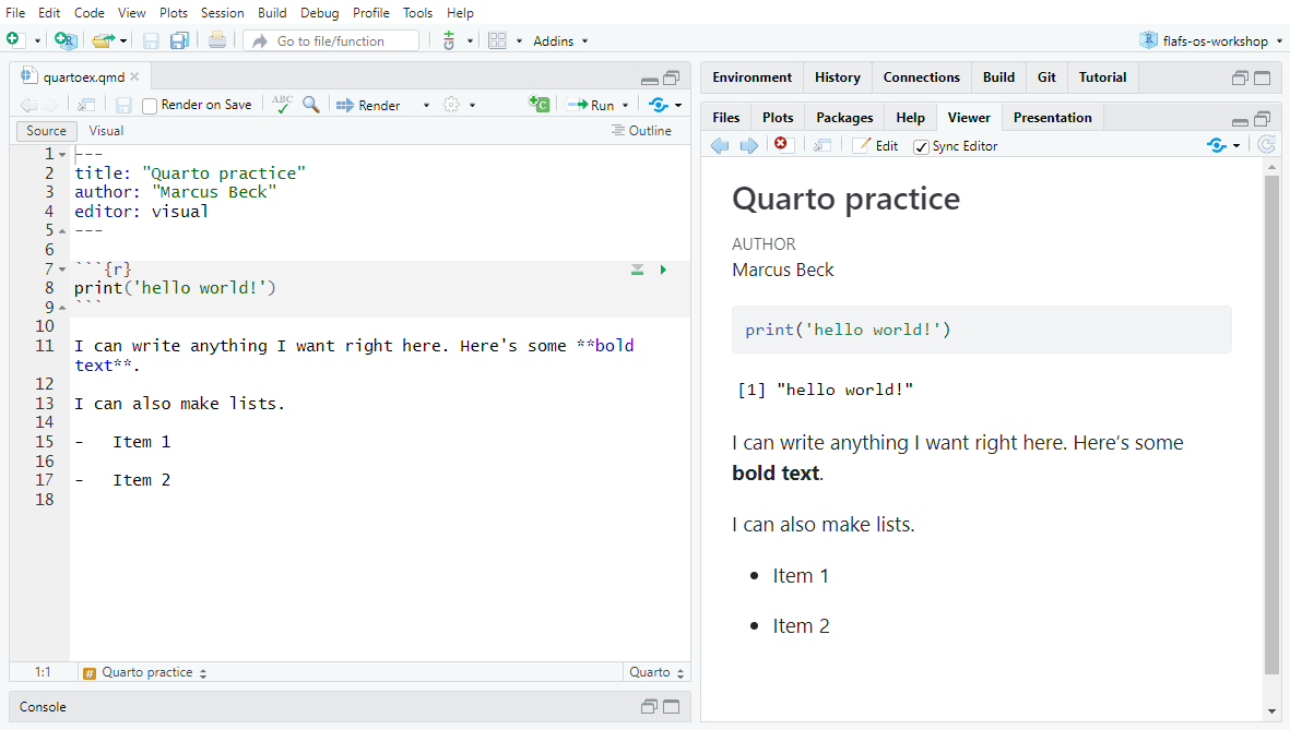
   Here’s what your RStudio session should look like (note the three parts of the source .qmd document - YAML, code chunk, and Markdown text). The rendered HTML file will appear in the Viewer pane on the right.

   

   Tip

   A rendered Quarto document as an HTML, PDF, Word, or other file format is stand-alone and can be shared with anybody!

Exercise

Repeat the above steps to create an RStudio project and Quarto file.

1. Create an RStudio project (skip if using Posit Cloud)
2. Open a new Quarto file
3. Create a code chunk and add some R code
4. Add some Markdown text outside of the code chunk
5. Render your document to marvel at your work

Answers

This is an example of what your Quarto file might look like:

---
title: "Quarto practice"
author: "Marcus Beck"
editor: visual
---

I  can write anything I want right here. Here's some **bold text**.
    
I can also make lists
    
1. Item 1
1. Item 2
    
```{r}
#| echo: true
print('Hello Quarto!')
```

2.3 Code chunk options

The behavior of the code chunks when the file is rendered can be changed using the many options available in Quarto. This can be useful for a few reasons.

1. Only displaying the output of a code chunk (e.g., a plot)
2. Only displaying the code and not running the chunk
3. Running the code without displaying output for use in other parts of the document
4. Suppressing warnings and messages
5. Defining table or figure options (e.g., height, width, captions, etc.)

Code chunk options can be applied globally to all chunks in the document or separately for each chunk.

To apply them globally, they’ll look something like this in the YAML, where options are added after execute:

---
title: "My Document"

execute: 
  echo: false
  warning: false
---

Tip

Be careful with indentation in the YAML, the document won’t render if the indentation is incorrect.

To apply to individual code chunks, use the #| (hashpipe) notation at the top of the code chunk. This will override any global options if you’ve included them in the top YAML. Below, echo: true indicates that the code will be displayed in the rendered output.

```{r}
#| echo: true
plot(1:10)
```

Here’s a short list of other useful execution options:

Option	Description
eval	Evaluate the code chunk (if false, just echos the code into the output).
echo	Include the source code in output
output	Include the results of executing the code in the output (true, false, or asis to indicate that the output is raw markdown and should not have any of Quarto’s standard enclosing markdown).
warning	Include warnings in the output.
error	Include errors in the output (note that this implies that errors executing code will not halt processing of the document).
include	Catch all for preventing any output (code or results) from being included (e.g. include: false suppresses all output from the code block).
message	Include messages in rendered output

R code can also be executed “inline” outside of code chunks. This can be useful if you want to include statements that reference particular values or information that is linked directly to data. Inline R code is entered using the r syntax followed by code.

I can enter inline text like `r 1 + 1`.

Text with inline R code will look like this when the document is rendered.

I can enter inline text like 2.

2.4 Figures and tables

Figures and tables are easily added in Quarto, created using R code or importing from an external source.

Any figures created in code chunks will be included in the rendered output. Some relevant code chunk options for figures include fig-height, fig-width, fig-cap, label (for cross-referencing) and fig-align.

```{r}
#| label: fig-myhist
#| fig-height: 4
#| fig-width: 6
#| fig-cap: "Here's my awesome histogram."
#| fig-align: "center"
vals <- rnorm(100)
hist(vals)
```

vals <- rnorm(100)
hist(vals)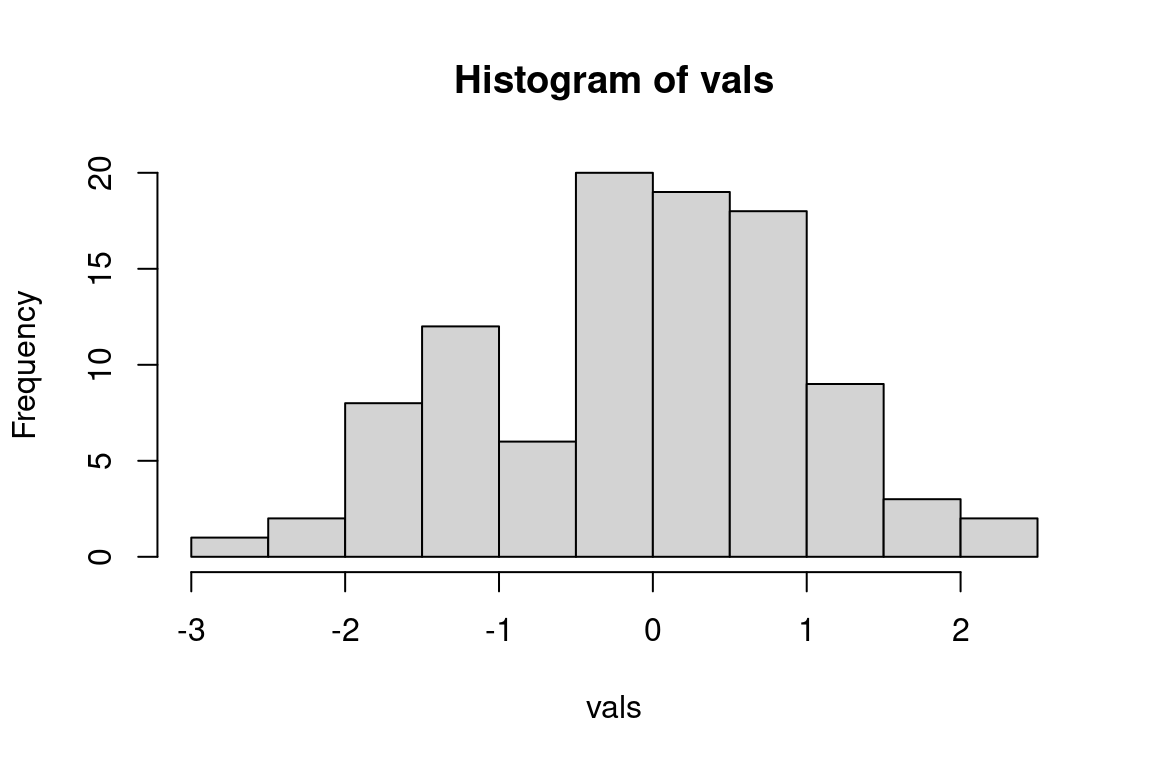

Figure 2.1: Here’s my awesome histogram.

Figures can be cross-referenced in the text using the @ notation with the figure label.

Here's a cross-reference to @fig-myhist.

When the file is rendered, the appropriate figure number will be displayed with a link to the figure:

Here’s a cross-reference to Figure 2.1.

Similarly, tabular output can be created inside code chunks.

```{r}
#| label: tbl-mytable
#| tbl-cap: "Here's my awesome table."
totab <- data.frame(
  Species = c('Oysters', 'Seagrass', 'Sand'),
  Count = c(12, 5, 4)
)
knitr::kable(totab)
```

totab <- data.frame(
  Species = c('Oysters', 'Seagrass', 'Sand'),
  Count = c(12, 5, 4)
)
knitr::kable(totab)

Table 2.1: Here’s my awesome table.

Species	Count
Oysters	12
Seagrass	5
Sand	4

And a cross-reference:

Here's a cross-reference to @tbl-mytable.

Here’s a cross-reference to Table 2.1.

Tip

Label tags for tables and figures must include the tbl- or fig- prefix for proper cross-referencing.

Figures can also be imported from an external source (e.g., from your computer or the web) using the ![]() notation. You can also simply add a figure from the file menu using the Visual editor.

![](figs/quarto/oysters.jpg)

You can also add a figure from a URL using the same notation.

![](https://unsplash.com/photos/HH-MuVCKal0)

Adding captions and labels to external figures looks something like this:

![Here are some beautiful oysters.](figs/quarto/oysters.jpg){#fig-oysters}

Figure 2.2: Here are some beautiful oysters.

The cross-reference is done the same.

Here's a cross-reference to @fig-oysters

Here's a cross-reference to Figure 2.2.

Likewise, tables can be imported from an external source (e.g., Excel). You’ll want to do this in a code chunk and add the appropriate options (e.g., to cross-reference Table 2.2).

```{r}
#| label: tbl-habitats
#| tbl-cap: "The first six rows of our tidy data"
mytab <- readxl::read_excel('data/tidy.xlsx')[1:6, ]
knitr::kable(mytab)
```

mytab <- readxl::read_excel('data/tidy.xlsx')[1:6, ]
knitr::kable(mytab)

Table 2.2: The first six rows of our tidy data

Location	Habitat	Year	Acres	Category
Clear Bay	Seagrass	2019	519	B
Clear Bay	Oysters	2019	390	B
Clear Bay	Sand	2019	742	C
Fish Bay	Seagrass	2019	930	B
Fish Bay	Oysters	2019	680	A
Fish Bay	Sand	2019	611	A

Visit these links for full details on figures and tables in Quarto. R also has a rich library of packages for producing tables, most of which play nice with Quarto.

Exercise

Create some tables, figures, and cross-references as above.

1. In the same file from the first exercise, create a code chunk and add some R code to create a simple plot (e.g., hist(mtcars$mpg))
2. Give the code chunk a label and figure caption
3. Use the figure label to add a cross-reference outside of the code chunk
4. Repeat the above, but this time create a table (e.g., knitr::kable(mtcars))
5. Render your document to marvel at your work

Answers

This is an example of what your Quarto file might look like:

---
title: "Quarto practice"
author: "Marcus Beck"
editor: visual
---

I  can write anything I want right here. Here's some **bold text**.
    
I can also make lists
    
1. Item 1
1. Item 2
    
```{r}
#| echo: true
print('Hello Quarto!')
```

@fig-myhist shows an awesome histogram. 

```{r}
#| label: fig-myhist
#| fig-cap: "Here's my awesome histogram."
hist(mtcars$mpg)
```

@tbl-mytable shows an awesome table. 

```{r}
#| label: tbl-mytable
#| tbl-cap: "Here's my awesome table."
knitr::kable(mtcars)
```

2.5 Quarto using htmlwidgets

The htmlwidgets package allows you to embed dynamic components directly into a Quarto HTML page. There are several packages that use htmlwidgets to automatically embed the required JavaScript visualization libraries. This does not require any knowledge of JavaScript, nor use of a Shiny Server.

2.5.1 leaflet

The leaflet package can be used to create interactive maps (also see mapview for an “out-of-the-box” option). Here’s a quick map of where we are - click on the marker to view the popup.

library(leaflet)

leaflet() %>%
  addTiles() %>%  # Add default basemap tiles
  addMarkers(lng = -122.663, lat = 45.529, popup = "CERF 2023 conference")

2.5.2 plotly and dygraphs

The plotly and dygraphs packages allow you to create interactive plots. They provide similar functionality, but serve different purposes.

library(plotly)
library(tibble)

# data to plot
toplo <- tibble(
  Species = c('Oysters', 'Seagrass', 'Sand'),
  `Clear Bay` = c(12, 5, 4), 
  `Fish Bay` = c(6, 7, 9)
)

# make a plotly plot
fig <- plot_ly(toplo, x = ~Species, y = ~`Clear Bay`, type = 'bar', name = 'Clear Bay')
fig <- fig %>% add_trace(y = ~`Fish Bay`, name = 'Fish Bay')
fig <- fig %>% layout(yaxis = list(title = 'Count'), barmode = 'group')

fig

The plotly package has an additional feature that can easily transform existing ggplot objects into plotly objects using the ggplotly() function. This works fairly well for simple plots, although it is usually a better option to build plotly plots from scratch.

library(ggplot2)
library(tidyr)

# data to plot
toplo <- tibble(
    Species = c('Oysters', 'Seagrass', 'Sand'),
    `Clear Bay` = c(12, 5, 4), 
    `Fish Bay` = c(6, 7, 9)
  ) %>% 
  pivot_longer(-Species, names_to = 'Bay', values_to = 'Count')

# make a ggplot
fig <- ggplot(toplo, aes(x = Species, y = Count, fill = Bay)) + 
  geom_bar(stat = 'identity', position = 'dodge')

# conver to plotly
ggplotly(fig)

Plotly also works well for three-dimensional plotting. Here we show a bathymetric map of Tampa Bay. The input file is a raster object converted to a matrix (see here)

library(plotly)

# file created from a DEM, see 
load(file = 'data/demmat.RData')

plot_ly(z = ~demmat) %>% 
  add_surface(colorbar = list(title = 'Depth (m)')) 

We can change some of the options using the layout() function. The aspect ratio, grid lines, and axis labels are all changed by created a list() object to pass to layout(). The color is changed in the add_surface() function (options here).

# setup plot options
axopt <- list(showgrid = F, title = '', 
              zerolinecolor='rgb(255, 255, 255)', 
              tickvals = NA)
scene <- list(
  aspectmode = 'manual', 
  aspectratio = list(x = 0.7, y = 1, z = 0.1),
  xaxis = axopt, yaxis = axopt, zaxis = axopt
  )

# create plot
plot_ly(z = ~demmat) %>% 
  add_surface(colorbar = list(title = 'Depth (m)'), colorscale = 'Jet', 
              reversescale = T) %>% 
  layout(scene = scene)

The dygraphs package is designed for time series data. First, we create a time series with random data, then plot it with dygraphs with a range selector.

library(dygraphs)

# create data
n <- 1000
y <- cumsum(rnorm(n))
dts <- seq.Date(Sys.Date(), by = 'day', length.out = n)
toplo <- tibble(
  Date = dts, 
  y = y
)

dygraph(toplo) %>% 
  dyRangeSelector()

Exercise

Add some htmlwidgets to your Quarto document.

1. Create a code chunk and add some code to produce a leaflet map. You can use the same lat/lon coordinates from above or pick your own from Google Maps. Install the leaflet package if you need to.
2. Create another code chunk and add some code to create a dygraph object. You can use the same code from above or create your own time series. Install the dygraphs package if you need to.
3. Render your document to marvel at your work

Answers

This is an example of what your Quarto file might look like:

---
title: "Quarto practice"
author: "Marcus Beck"
editor: visual
---

```{r}
#| echo: false
#| message: false
library(leaflet)
library(dygraphs)
library(tibble)
```

I  can write anything I want right here. Here's some **bold text**.
    
I can also make lists
    
1. Item 1
1. Item 2
    
```{r}
#| echo: true
print('Hello Quarto!')
```

@fig-myhist shows an awesome histogram. 

```{r}
#| label: fig-myhist
#| fig-cap: "Here's my awesome histogram."
hist(mtcars$mpg)
```

@tbl-mytable shows an awesome table. 

```{r}
#| label: tbl-mytable
#| tbl-cap: "Here's my awesome table."
knitr::kable(mtcars)
```

```{r}
leaflet() %>% 
  addTiles() %>% 
  addMarkers(lng = -82.5, lat = 27.5)
```

```{r}
# create data
n <- 1000
y <- cumsum(rnorm(n))
dts <- seq.Date(Sys.Date(), by = 'day', length.out = n)
toplo <- tibble(
  Date = dts, 
  y = y
)

dygraph(toplo) %>% 
  dyRangeSelector()
```

2.6 Quarto using crosstalk

The crosstalk package can incorporate additional dynamic functionality in a Quarto document. As the name implies, it allows linking between plots and tables by including embedded Javascript in the rendered HTML file. This allows functionality that looks interactive as in a Shiny application, but does not require Shiny Server.

library(crosstalk)
library(leaflet)
library(DT)
library(dplyr)

# import water quality data
tbwqdat <- read.csv('https://github.com/tbep-tech/shiny-workshop/raw/main/data/tbwqdat.csv') %>% 
  filter(mo == 7)

# create shared data
sd <- SharedData$new(tbwqdat)

# create a filter input
filter_slider("chla", "Chlorophyll-a", sd, column=~chla, step=0.1, width=250)

# use shared data with crosstalk widgets
bscols(
  leaflet(sd) %>% 
    addTiles() %>% 
    addMarkers(),
  datatable(
    sd, extensions = "Scroller", style="bootstrap", class = "compact", width = "100%", rownames = F,
    options =list(
      scrollY = 300, scroller = TRUE, 
      columnDefs = list(
        list(visible = F, targets = c(0:1, 4)),
         list(className = 'dt-left', targets = '_all'))
      ),
      colnames = c('lat', 'lon', 'Bay segment', 'Station', 'mo', 'Chl-a (ug/L)')
    )
  )

Chlorophyll-a

2.7 Quarto using Observable

Observable is a relatively new approach that also allows dynamic features to be included in a Quarto document. It is an entirely separate language outside of R that uses JavaScript and allows excellent functionality similar what is provided by a Shiny Server. The following plot shows a histogram of chlorophyll values by bay segment that is created using the code below.

datatr = transpose(data)
filtered = datatr.filter(function(dat) {
  return chla < dat.chla &&
    bay_segment.includes(dat.bay_segment) ;
})
viewof chla = Inputs.range(
  [1.3, 66.6], 
  {value: 1.3, step: 1, label: "Chlorophyll-a (ug/L):"}
)
viewof bay_segment = Inputs.checkbox(
  ["OTB", "HB", "MTB", "LTB"], 
  { value: ["OTB", "HB", "MTB", "LTB"], 
    label: "Bay segments:"
  }
)
Plot.rectY(filtered, 
  Plot.binX(
    {y: "count"}, 
    {x: "chla", thresholds: 10, fill: "bay_segment"}
  ))
  .plot({
    x: {label: "Chlorophyll-a"},
    color: {legend: true},
    marks: [
      Plot.frame(),
    ]
  }
)

First, import the data as you would in R, then define variables for Observable using ojs_define(). Note that Observable code chunks cannot be run interactively and only work when an entire Quarto document is rendered.

# import water quality data
tbwqdat <- readr::read_csv('https://github.com/tbep-tech/shiny-workshop/raw/main/data/tbwqdat.csv')

# define variables
ojs_define(data = tbwqdat)

Then we create some selector widgets to filter by the range of chlorophyll values and data by individual bay segments.

```{ojs}
viewof chla = Inputs.range(
  [1.8, 17.4], 
  {value: 1.8, step: 1, label: "Chlorophyll-a (ug/L):"}
)
viewof bay_segment = Inputs.checkbox(
  ["OTB", "HB", "MTB", "LTB"], 
  { value: ["OTB", "HB", "MTB", "LTB"], 
    label: "Bay segments:"
  }
)
```

A filtering function is then created to filter the data based on the selections from the widget. Note use of the transpose() function. This is required to use R data in a row/column format to an array format used in a JavaScript setting.

```{ojs}
datatr = transpose(data)
filtered = datatr.filter(function(dat) {
  return chla < dat.chla &&
    bay_segment.includes(dat.bay_segment) ;
})
```

Finally, we create the plot using the filtered data function.

```{ojs}
Plot.rectY(filtered, 
  Plot.binX(
    {y: "count"}, 
    {x: "chla", thresholds: 10, fill: "bay_segment"}
  ))
  .plot({
    x: {label: "Chlorophyll-a"},
    color: {legend: true},
    marks: [
      Plot.frame(),
    ]
  }
)
```

Additional information on using Observable with Quarto is available here.

2.8 Sharing HTML files

An advantage of creating a dynamic HTML file with Quarto is the ability to share it with anybody. An HTML file can easily be shared by email, although it must be created as a “standalone” file for others to use. You’ll notice that sometimes external files or subfolders are created when you use any of the above options to add dynamic content. This is fine if you are working locally, but to share with others, you can create a standalone HTML file by adding the following option in the YAML:

format:
  html:
    embed-resources: true

2.9 Publishing

A rendered HTML file can also be hosted online and shared by URL. This approach is useful to make the document available to anyone with the web address.

The easiest way to do this is to publish your document to RPubs, a free service from Posit for sharing web documents. Click the publish button on the top-right of the editor toolbar. You will be prompted to create an account if you don’t have one already.

This can also be done using the quarto R package in the console.

quarto::quarto_publish_doc(
  "data/quartoex.qmd", 
  server = "rpubs.com"
  )

You can also use the Quarto CLI in the terminal. Here we are publishing the document to Quarto Pub.

Terminal

quarto publish quarto-pub data/quartoex.qmd

If your Quarto document is in an RStudio project on GitHub, you can also publish to GitHub Pages.

Terminal

quarto publish gh-pages data/quartoex.qmd

Exercise

Publish your Quarto document using any of the methods above (bonus points if you use GitHub).

2.10 Summary

In this module we learned the basics of creating dynamic documents with Quarto that combine markdown text with R code. There’s much, much more Quarto can do for you. Please visit https://quarto.org/ for more information on how you can use these documents to fully leverage their potential for open science.

Knuth, Donald E. 1984. “Literate Programming.” Comput. J. 27 (2): 97–111. https://doi.org/10.1093/comjnl/27.2.97.