# install
install.packages('tidyverse')2 Data wrangling part 1
Get the lesson R script: data_wrangling_1.R
Get the lesson data: download zip
2.1 Lesson Outline
2.2 Lesson Exercises
2.3 Goals
Data wrangling (cleaning, manipulation, ninjery, etc.) is the part of any data analysis that will take the most time. While it may not be fun, it is necessary for the work that follows. I strongly believe that mastering these skills has more value than mastering a particular analysis. Check out this article if you don’t believe me.
We’ll have two hours to cover parts 1 and 2 of data wrangling. It’s unrealistic to expect that you will be a ninja wrangler after this training. As such, the goals are to expose you to fundamentals and to develop an appreciation of what’s possible. I’ll also provide resources that you can use for follow-up learning on your own.
After this lesson you should be able to answer (or be able to find answers to) the following:
- Why do we need to manipulate data?
- What is the tidyverse?
- What can you do with dplyr?
- What is piping?
2.4 The tidyverse
The tidyverse is a set of packages that work in harmony because they share common data representations and design. The tidyverse package is designed to make it easy to install and load core packages from the tidyverse in a single command. With tidyverse, you’ll be able to address all steps of data exploration.
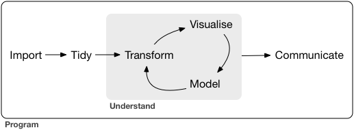
From the excellent book, R for Data Science (2nd Ed.), data exploration is the art of looking at your data, rapidly generating hypotheses, quickly testing them, then repeating again and again and again. Tools in the tidyverse also have direct application to more formal analyses with many of the other available R packages on CRAN.
You should already have the tidyverse installed, but let’s give it a go if you haven’t done this part yet:
After installation, we can load the package:
# load
library(tidyverse)
── Attaching core tidyverse packages ──────────────────────── tidyverse 2.0.0 ──
✔ dplyr 1.2.1 ✔ readr 2.2.0
✔ forcats 1.0.1 ✔ stringr 1.6.0
✔ ggplot2 4.0.3 ✔ tibble 3.3.1
✔ lubridate 1.9.5 ✔ tidyr 1.3.2
✔ purrr 1.2.2
── Conflicts ────────────────────────────────────────── tidyverse_conflicts() ──
✖ dplyr::filter() masks stats::filter()
✖ dplyr::lag() masks stats::lag()
ℹ Use the conflicted package (<http://conflicted.r-lib.org/>) to force all conflicts to become errorsNotice that the messages you get after loading are a bit different from other packages. That’s because tidyverse is a package that manages other packages (this is the only package I know of that serves this function). Loading tidyverse will load all of the core packages:
- ggplot2 for data visualisation
- dplyr for data manipulation
- tidyr for data tidying
- readr for data import
- purrr for functional programming
- tibble for tibbles, a modern re-imagining of data frames
- stringr for working with text strings
- forcats for working with factors
- lubridate for working with dates and times
Other packages (e.g., readxl) are also included but you will probably not use these as frequently.
A nice feature of tidyverse is the ability to check for and install new versions of each package:
tidyverse_update()
#> The following packages are out of date:
#>
#> • dbplyr        (2.3.2 -> 2.6.0)
#> • rlang         (1.1.7 -> 1.2.0)
#> • tibble        (3.2.1 -> 3.3.1)
#> • xml2          (1.5.2 -> 1.6.0)
#>
#> Start a clean R session then run:
#> install.packages(c("dbplyr", "rlang", "tibble", "xml2"))
As you’ll soon learn using R, there are often several ways to achieve the same goal. The tidyverse provides tools to address problems that can be solved with other packages or even functions from the base installation. Tidyverse is admittedly an opinionated approach to data exploration, but it’s popularity and rapid growth within the R community is a testament to the power of the tools that are provided.
2.5 Data wrangling with dplyr
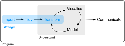
The data wrangling process includes data import, tidying, and transformation. The process directly feeds into, and is not mutually exclusive with, the understanding or modelling side of data exploration. More generally, I consider data wrangling as the manipulation or combination of datasets for the purpose of analysis.
Wrangling begins with import and ends with an output of some kind that is ready for analysis, such as a plot or a model. In a perfect world, the wrangling process is linear with no need for back-tracking. In reality, we often uncover more information about a dataset, either through wrangling or modeling, that warrants re-evaluation or even gathering more data. Data also come in many forms and the form you need for analysis is rarely the required form of the input data. For these reasons, data wrangling will consume most of your time in data exploration.
All wrangling is based on a purpose. No one wrangles for the sake of wrangling (usually), so the process always begins by answering the following two questions:
- What do my input data look like?
- What should my input data look like given what I want to do?
At the most basic level, going from what your input data looks like to what it needs to look like will require a few key operations. Some common examples:
- Selecting specific variables (columns)
- Filtering observations (rows) by some criteria
- Adding or modifying existing variables
- Renaming variables
- Arranging rows by a variable
- Summarizing variables conditional on others
The dplyr package provides easy tools for these common data manipulation tasks. It is built to work directly with data frames and is one of the most heavily used packages in the tidyverse. The philosophy of dplyr is that one function does one thing and the name of the function says what it does. This is where the tidyverse generally departs from other packages and even base R. It is meant to be easy, logical, and intuitive. There is a lot of great info on dplyr. If you have an interest, I’d encourage you to look more. The vignettes are particularly good.
I’ll demonstrate the examples with the training dataset from the last lesson.
library(here)

# import the data
metadat <- read_csv(here('data', 'metadat.csv'))

# see first six rows
head(metadat)
# A tibble: 6 × 73
station_no station_name station_latitude station_longitude Waterbody_Name
<dbl> <chr> <dbl> <dbl> <chr>
1 23144 Lake Panasoffkee… 28.8 -82.1 Lake Panasoff…
2 23169 Lake Panasoffkee… 28.8 -82.2 Lake Panasoff…
3 23113 Lake Panasoffkee… 28.8 -82.1 Lake Panasoff…
4 23152 Lake Panasoffkee… 28.8 -82.1 Lake Panasoff…
5 1035944 Lake Panasoffkee… 28.8 -82.1 Lake Panasoff…
6 23167 Lake Panasoffkee… 28.8 -82.2 Lake Panasoff…
# ℹ 68 more variables: station_elevation <dbl>, WBID_Plan_Unit <chr>,
# hydrounit_name <chr>, WBID_Class <dbl>, SWF_Parcel_No <chr>,
# station_status_remark <chr>, WBID <chr>, hydrounit_title <chr>,
# Co_Parcel_No <chr>, ngr_letter <chr>, Sec_Twn_Rng <chr>,
# WQ_Instrumentation <lgl>, admin_level <chr>, catchment_size <dbl>,
# Station_ZIP_Code <dbl>, Station_Owner <chr>, region_township <chr>,
# Station_Characteristic <chr>, Hydrologic_Data_Priority_Station <chr>, …# dimensions
dim(metadat)[1] 8 73# column names
names(metadat) [1] "station_no" "station_name"
[3] "station_latitude" "station_longitude"
[5] "Waterbody_Name" "station_elevation"
[7] "WBID_Plan_Unit" "hydrounit_name"
[9] "WBID_Class" "SWF_Parcel_No"
[11] "station_status_remark" "WBID"
[13] "hydrounit_title" "Co_Parcel_No"
[15] "ngr_letter" "Sec_Twn_Rng"
[17] "WQ_Instrumentation" "admin_level"
[19] "catchment_size" "Station_ZIP_Code"
[21] "Station_Owner" "region_township"
[23] "Station_Characteristic" "Hydrologic_Data_Priority_Station"
[25] "Datum_Shift_Derivation" "WMD"
[27] "station_catchment_area" "Equipment_Owner2"
[29] "WQMP_Sampled" "SW_High_Threshold_29"
[31] "GARR_Cell_ID" "WBID_Waterbody"
[33] "SW_Low_Threshold_29" "MFL_Rule"
[35] "Instrumentation" "Station_Town_City"
[37] "FGS_ID" "Legacy_ID"
[39] "County" "Instrumentation2"
[41] "Station_Type_Surfacewater" "DMIT"
[43] "USGS_ID_Number" "Gauge_Datum_Description"
[45] "Land_Surface_Elevation_NAVD88" "Local_Stn_Name"
[47] "FDEP_ID" "Equipment_Owner"
[49] "station_status" "CFWI"
[51] "USGS_Station_Name" "Access_Agreement_Flag"
[53] "Guidance_Levels" "WBID_Update"
[55] "Station_Type" "TBW_Stn_Name"
[57] "admin_name" "USGS_Primary_Basin"
[59] "Hydrologic_Data_Region" "SW_High_Threshold_88"
[61] "Shift_Date_Time" "station_gauge_datum_remark"
[63] "GAUGE_DATUM" "Gauge_Datum_Correction"
[65] "SW_Low_Threshold_88" "Datum_Shift_Value"
[67] "station_gauge_datum" "station_gauge_datum_unit"
[69] "Gauge_Datum_Correction_29" "SW_DID1"
[71] "station_gauge_datum_from" "hydrounit_no"
[73] "region_district" # structure
str(metadat)spc_tbl_ [8 × 73] (S3: spec_tbl_df/tbl_df/tbl/data.frame)
$ station_no : num [1:8] 23144 23169 23113 23152 1035944 ...
$ station_name : chr [1:8] "Lake Panasoffkee 1" "Lake Panasoffkee 4" "Lake Panasoffkee 7" "Lake Panasoffkee 8" ...
$ station_latitude : num [1:8] 28.8 28.8 28.8 28.8 28.8 ...
$ station_longitude : num [1:8] -82.1 -82.2 -82.1 -82.1 -82.1 ...
$ Waterbody_Name : chr [1:8] "Lake Panasoffkee" "Lake Panasoffkee" "Lake Panasoffkee" "Lake Panasoffkee" ...
$ station_elevation : num [1:8] 38.2 39.3 38.2 38.2 NA ...
$ WBID_Plan_Unit : chr [1:8] "Lake Panasoffkee" "Lake Panasoffkee" "Lake Panasoffkee" "Lake Panasoffkee" ...
$ hydrounit_name : chr [1:8] "HUC12" "HUC12" "HUC12" "HUC12" ...
$ WBID_Class : num [1:8] 3 3 3 3 3 3 3 3
$ SWF_Parcel_No : chr [1:8] "---" "---" "---" "---" ...
$ station_status_remark : chr [1:8] NA NA NA NA ...
$ WBID : chr [1:8] "1351B" "1351C" "1351B" "1351B" ...
$ hydrounit_title : chr [1:8] "HUC 12" "HUC 12" "HUC 12" "HUC 12" ...
$ Co_Parcel_No : chr [1:8] "F03-1000" "Water" "J34-1000" "F03-1000" ...
$ ngr_letter : chr [1:8] "-" "-" "-" "-" ...
$ Sec_Twn_Rng : chr [1:8] "29 19 22" "30 19 22" "04 20 22" "19 19 22" ...
$ WQ_Instrumentation : logi [1:8] NA NA NA NA NA NA ...
$ admin_level : chr [1:8] "Sub district" "Sub district" "Sub district" "Sub district" ...
$ catchment_size : num [1:8] 19979 19979 19979 19979 NA ...
$ Station_ZIP_Code : num [1:8] 34785 33538 33538 34785 34785 ...
$ Station_Owner : chr [1:8] "Southwest Florida Water Management District" "Southwest Florida Water Management District" "Southwest Florida Water Management District" "Southwest Florida Water Management District" ...
$ region_township : chr [1:8] "Northern Planning Region" "Northern Planning Region" "Northern Planning Region" "Northern Planning Region" ...
$ Station_Characteristic : chr [1:8] "Surface Water" "Surface Water" "Surface Water" "Surface Water" ...
$ Hydrologic_Data_Priority_Station: chr [1:8] "no" "no" "no" "no" ...
$ Datum_Shift_Derivation : chr [1:8] NA NA NA NA ...
$ WMD : chr [1:8] "SWFWMD" "SWFWMD" "SWFWMD" "SWFWMD" ...
$ station_catchment_area : num [1:8] 19979 19979 19979 19979 NA ...
$ Equipment_Owner2 : chr [1:8] NA NA NA NA ...
$ WQMP_Sampled : chr [1:8] "yes" "yes" "yes" "yes" ...
$ SW_High_Threshold_29 : num [1:8] NA NA NA NA NA NA 0 50
$ GARR_Cell_ID : chr [1:8] "120727" "120252" "119780" "121201" ...
$ WBID_Waterbody : chr [1:8] "LAKE PANASOFFKEE" "OUTLET RIVER" "LAKE PANASOFFKEE" "LAKE PANASOFFKEE" ...
$ SW_Low_Threshold_29 : num [1:8] NA NA NA NA NA NA 0 0
$ MFL_Rule : chr [1:8] "no" "no" "no" "no" ...
$ Instrumentation : chr [1:8] "Staff Gauge" "Staff Gauge" "Staff Gauge" "Staff Gauge" ...
$ Station_Town_City : chr [1:8] "Wildwood" "Lake Panasoffkee" "Lake Panasoffkee" "Wildwood" ...
$ FGS_ID : chr [1:8] "---" "---" "---" "---" ...
$ Legacy_ID : chr [1:8] "S0130300" "S0130400" "S0130500" "S0130600" ...
$ County : chr [1:8] "Sumter" "Sumter" "Sumter" "Sumter" ...
$ Instrumentation2 : chr [1:8] NA NA NA NA ...
$ Station_Type_Surfacewater : chr [1:8] "Lake" "Lake" "Lake" "Lake" ...
$ DMIT : chr [1:8] "no" "no" "no" "no" ...
$ USGS_ID_Number : chr [1:8] "---" "---" "---" "---" ...
$ Gauge_Datum_Description : chr [1:8] NA NA NA NA ...
$ Land_Surface_Elevation_NAVD88 : num [1:8] 38.2 39.3 38.2 38.2 NA ...
$ Local_Stn_Name : chr [1:8] "---" "---" "---" "---" ...
$ FDEP_ID : chr [1:8] "284817082092701" "284804082090501" "284637082063501" "284921082081801" ...
$ Equipment_Owner : chr [1:8] "Southwest Florida Water Management District" "Southwest Florida Water Management District" "Southwest Florida Water Management District" "Southwest Florida Water Management District" ...
$ station_status : chr [1:8] "Active" "Active" "Active" "Active" ...
$ CFWI : chr [1:8] "no" "no" "no" "no" ...
$ USGS_Station_Name : chr [1:8] "---" "---" "---" "---" ...
$ Access_Agreement_Flag : chr [1:8] "no" "no" "no" "no" ...
$ Guidance_Levels : chr [1:8] "no" "no" "no" "no" ...
$ WBID_Update : POSIXct[1:8], format: "2020-11-20" "2020-11-20" ...
$ Station_Type : chr [1:8] "Lake" "Lake" "Lake" "Lake" ...
$ TBW_Stn_Name : logi [1:8] NA NA NA NA NA NA ...
$ admin_name : chr [1:8] "Northern Planning Region" "Northern Planning Region" "Northern Planning Region" "Northern Planning Region" ...
$ USGS_Primary_Basin : logi [1:8] NA NA NA NA NA NA ...
$ Hydrologic_Data_Region : chr [1:8] "---" "---" "---" "---" ...
$ SW_High_Threshold_88 : num [1:8] NA NA NA NA 44.1 ...
$ Shift_Date_Time : POSIXct[1:8], format: NA NA ...
$ station_gauge_datum_remark : chr [1:8] NA NA NA NA ...
$ GAUGE_DATUM : num [1:8] NA NA NA NA 0 NA NA 0
$ Gauge_Datum_Correction : num [1:8] NA NA NA NA 0 NA NA 0
$ SW_Low_Threshold_88 : num [1:8] NA NA NA NA 35.4 NA NA 35.5
$ Datum_Shift_Value : num [1:8] NA NA NA NA -0.85 NA NA -0.85
$ station_gauge_datum : num [1:8] NA NA NA NA 0 NA NA 0
$ station_gauge_datum_unit : chr [1:8] NA NA NA NA ...
$ Gauge_Datum_Correction_29 : num [1:8] NA NA NA NA NA NA NA 0
$ SW_DID1 : num [1:8] NA NA NA NA 0 NA NA 0
$ station_gauge_datum_from : num [1:8] NA NA NA NA 1.74e+12 ...
$ hydrounit_no : chr [1:8] NA NA NA NA ...
$ region_district : chr [1:8] NA NA NA NA ...
- attr(*, "spec")=
.. cols(
.. station_no = col_double(),
.. station_name = col_character(),
.. station_latitude = col_double(),
.. station_longitude = col_double(),
.. Waterbody_Name = col_character(),
.. station_elevation = col_double(),
.. WBID_Plan_Unit = col_character(),
.. hydrounit_name = col_character(),
.. WBID_Class = col_double(),
.. SWF_Parcel_No = col_character(),
.. station_status_remark = col_character(),
.. WBID = col_character(),
.. hydrounit_title = col_character(),
.. Co_Parcel_No = col_character(),
.. ngr_letter = col_character(),
.. Sec_Twn_Rng = col_character(),
.. WQ_Instrumentation = col_logical(),
.. admin_level = col_character(),
.. catchment_size = col_double(),
.. Station_ZIP_Code = col_double(),
.. Station_Owner = col_character(),
.. region_township = col_character(),
.. Station_Characteristic = col_character(),
.. Hydrologic_Data_Priority_Station = col_character(),
.. Datum_Shift_Derivation = col_character(),
.. WMD = col_character(),
.. station_catchment_area = col_double(),
.. Equipment_Owner2 = col_character(),
.. WQMP_Sampled = col_character(),
.. SW_High_Threshold_29 = col_double(),
.. GARR_Cell_ID = col_character(),
.. WBID_Waterbody = col_character(),
.. SW_Low_Threshold_29 = col_double(),
.. MFL_Rule = col_character(),
.. Instrumentation = col_character(),
.. Station_Town_City = col_character(),
.. FGS_ID = col_character(),
.. Legacy_ID = col_character(),
.. County = col_character(),
.. Instrumentation2 = col_character(),
.. Station_Type_Surfacewater = col_character(),
.. DMIT = col_character(),
.. USGS_ID_Number = col_character(),
.. Gauge_Datum_Description = col_character(),
.. Land_Surface_Elevation_NAVD88 = col_double(),
.. Local_Stn_Name = col_character(),
.. FDEP_ID = col_character(),
.. Equipment_Owner = col_character(),
.. station_status = col_character(),
.. CFWI = col_character(),
.. USGS_Station_Name = col_character(),
.. Access_Agreement_Flag = col_character(),
.. Guidance_Levels = col_character(),
.. WBID_Update = col_datetime(format = ""),
.. Station_Type = col_character(),
.. TBW_Stn_Name = col_logical(),
.. admin_name = col_character(),
.. USGS_Primary_Basin = col_logical(),
.. Hydrologic_Data_Region = col_character(),
.. SW_High_Threshold_88 = col_double(),
.. Shift_Date_Time = col_datetime(format = ""),
.. station_gauge_datum_remark = col_character(),
.. GAUGE_DATUM = col_double(),
.. Gauge_Datum_Correction = col_double(),
.. SW_Low_Threshold_88 = col_double(),
.. Datum_Shift_Value = col_double(),
.. station_gauge_datum = col_double(),
.. station_gauge_datum_unit = col_character(),
.. Gauge_Datum_Correction_29 = col_double(),
.. SW_DID1 = col_double(),
.. station_gauge_datum_from = col_double(),
.. hydrounit_no = col_character(),
.. region_district = col_character()
.. )
- attr(*, "problems")=<pointer: 0x55b108a01a30> 2.5.1 Selecting
Let’s begin using dplyr. Don’t forget to load the tidyverse if you haven’t done so already. We can use the select function to, you guessed it, select columns.
# first, select some columns
dplyr_sel1 <- select(metadat, station_no, station_name, station_latitude, station_longitude)
head(dplyr_sel1)
# A tibble: 6 × 4
station_no station_name station_latitude station_longitude
<dbl> <chr> <dbl> <dbl>
1 23144 Lake Panasoffkee 1 28.8 -82.1
2 23169 Lake Panasoffkee 4 28.8 -82.2
3 23113 Lake Panasoffkee 7 28.8 -82.1
4 23152 Lake Panasoffkee 8 28.8 -82.1
5 1035944 Lake Panasoffkee at CR 455 28.8 -82.1
6 23167 Lake Panasoffkee Outlet 28.8 -82.2# select everything but some columns
dplyr_sel2 <- select(metadat, -c(Waterbody_Name:region_district))
head(dplyr_sel2)# A tibble: 6 × 4
station_no station_name station_latitude station_longitude
<dbl> <chr> <dbl> <dbl>
1 23144 Lake Panasoffkee 1 28.8 -82.1
2 23169 Lake Panasoffkee 4 28.8 -82.2
3 23113 Lake Panasoffkee 7 28.8 -82.1
4 23152 Lake Panasoffkee 8 28.8 -82.1
5 1035944 Lake Panasoffkee at CR 455 28.8 -82.1
6 23167 Lake Panasoffkee Outlet 28.8 -82.2# select and rename
dplyr_sel3 <- select(metadat, number = station_no, name = station_name, station_latitude, station_longitude)
head(dplyr_sel3)# A tibble: 6 × 4
number name station_latitude station_longitude
<dbl> <chr> <dbl> <dbl>
1 23144 Lake Panasoffkee 1 28.8 -82.1
2 23169 Lake Panasoffkee 4 28.8 -82.2
3 23113 Lake Panasoffkee 7 28.8 -82.1
4 23152 Lake Panasoffkee 8 28.8 -82.1
5 1035944 Lake Panasoffkee at CR 455 28.8 -82.1
6 23167 Lake Panasoffkee Outlet 28.8 -82.22.5.2 Filtering
After selecting columns, you’ll probably want to remove or retain observations (rows) that fit some criteria. We’ll use the water quality data for this example.
# import water quality data
wqdat <- read_csv(here('data', 'wqdat.csv'))

# see first six rows
head(wqdat)
# A tibble: 6 × 7
station_no station_name parametertype_shortname parametertype_name
<dbl> <chr> <chr> <chr>
1 23113 Lake Panasoffkee 7 WQ_79 Alkalinity (CaCO3)
2 23113 Lake Panasoffkee 7 WQ_79 Alkalinity (CaCO3)
3 23113 Lake Panasoffkee 7 WQ_79 Alkalinity (CaCO3)
4 23113 Lake Panasoffkee 7 WQ_79 Alkalinity (CaCO3)
5 23113 Lake Panasoffkee 7 WQ_79 Alkalinity (CaCO3)
6 23113 Lake Panasoffkee 7 WQ_79 Alkalinity (CaCO3)
# ℹ 3 more variables: timestamp <dttm>, value <dbl>, unit_symbol <chr># dimensions
dim(wqdat)[1] 51931 7# column names
names(wqdat)[1] "station_no" "station_name"
[3] "parametertype_shortname" "parametertype_name"
[5] "timestamp" "value"
[7] "unit_symbol" # structure
str(wqdat)spc_tbl_ [51,931 × 7] (S3: spec_tbl_df/tbl_df/tbl/data.frame)
$ station_no : num [1:51931] 23113 23113 23113 23113 23113 ...
$ station_name : chr [1:51931] "Lake Panasoffkee 7" "Lake Panasoffkee 7" "Lake Panasoffkee 7" "Lake Panasoffkee 7" ...
$ parametertype_shortname: chr [1:51931] "WQ_79" "WQ_79" "WQ_79" "WQ_79" ...
$ parametertype_name : chr [1:51931] "Alkalinity (CaCO3)" "Alkalinity (CaCO3)" "Alkalinity (CaCO3)" "Alkalinity (CaCO3)" ...
$ timestamp : POSIXct[1:51931], format: "2000-11-08 11:30:00" "2000-11-08 11:30:00" ...
$ value : num [1:51931] 73 73 88.7 88.7 118 119 119 137 137 119 ...
$ unit_symbol : chr [1:51931] "mg/l" "mg/l" "mg/l" "mg/l" ...
- attr(*, "spec")=
.. cols(
.. station_no = col_double(),
.. station_name = col_character(),
.. parametertype_shortname = col_character(),
.. parametertype_name = col_character(),
.. timestamp = col_datetime(format = ""),
.. value = col_double(),
.. unit_symbol = col_character()
.. )
- attr(*, "problems")=<pointer: 0x55b104d052b0> Maybe you want to look at only one parameter.
# filter data for one parameter
wqdat_temp <- filter(wqdat, parametertype_name == "Temperature, Water")
head(wqdat_temp)
# A tibble: 6 × 7
station_no station_name parametertype_shortname parametertype_name
<dbl> <chr> <chr> <chr>
1 23113 Lake Panasoffkee 7 WQ_360 Temperature, Water
2 23113 Lake Panasoffkee 7 WQ_360 Temperature, Water
3 23113 Lake Panasoffkee 7 WQ_360 Temperature, Water
4 23113 Lake Panasoffkee 7 WQ_360 Temperature, Water
5 23113 Lake Panasoffkee 7 WQ_360 Temperature, Water
6 23113 Lake Panasoffkee 7 WQ_360 Temperature, Water
# ℹ 3 more variables: timestamp <dttm>, value <dbl>, unit_symbol <chr>dim(wqdat_temp)[1] 3350 7Or maybe you want to exclude data from one station.
# filter data to remove one station
wqdat_sta <- filter(wqdat, station_name != "Lake Panasoffkee 7")
head(wqdat_sta)
# A tibble: 6 × 7
station_no station_name parametertype_shortname parametertype_name
<dbl> <chr> <chr> <chr>
1 23144 Lake Panasoffkee 1 WQ_79 Alkalinity (CaCO3)
2 23144 Lake Panasoffkee 1 WQ_79 Alkalinity (CaCO3)
3 23144 Lake Panasoffkee 1 WQ_79 Alkalinity (CaCO3)
4 23144 Lake Panasoffkee 1 WQ_79 Alkalinity (CaCO3)
5 23144 Lake Panasoffkee 1 WQ_79 Alkalinity (CaCO3)
6 23144 Lake Panasoffkee 1 WQ_79 Alkalinity (CaCO3)
# ℹ 3 more variables: timestamp <dttm>, value <dbl>, unit_symbol <chr>dim(wqdat_sta)[1] 41185 7Filtering can take a bit of time to master because there are several ways to tell R what you want. Within the filter function, the working part is a logical selection of TRUE and FALSE values that are used to select rows (TRUE means I want that row, FALSE means I don’t). Every selection within the filter function, no matter how complicated, will always be a T/F vector. This is similar to running queries on a database if you’re familiar with SQL.
To use filtering effectively, you have to know how to select the observations you want using the comparison operators. R provides the standard suite: >, >=, <, <=, != (not equal), and == (equal). When you’re starting out with R, the easiest mistake to make is to use = instead of == when testing for equality.
Multiple logical selections to filter() can be combined. Every expression must be true in order for a row to be included in the output. You’ll need to use Boolean operators: & is “and”, | is “or”, and ! is “not”. This is the complete set of Boolean operations.
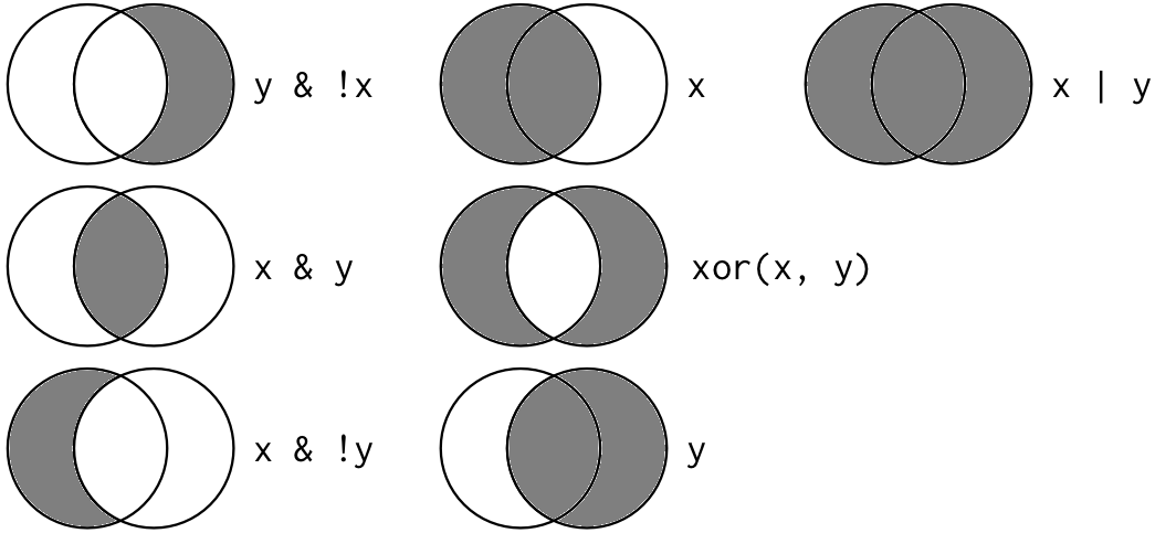
Let’s create some more complicated filtering examples.
# all rows with water temperature greater than 25 C
filt1 <- filter(wqdat, parametertype_name == 'Temperature, Water' & value > 25)
head(filt1)
# A tibble: 6 × 7
station_no station_name parametertype_shortname parametertype_name
<dbl> <chr> <chr> <chr>
1 23113 Lake Panasoffkee 7 WQ_360 Temperature, Water
2 23113 Lake Panasoffkee 7 WQ_360 Temperature, Water
3 23113 Lake Panasoffkee 7 WQ_360 Temperature, Water
4 23113 Lake Panasoffkee 7 WQ_360 Temperature, Water
5 23113 Lake Panasoffkee 7 WQ_360 Temperature, Water
6 23113 Lake Panasoffkee 7 WQ_360 Temperature, Water
# ℹ 3 more variables: timestamp <dttm>, value <dbl>, unit_symbol <chr># all rows with water temperature greater than 25 C and less than 30 C
filt2 <- filter(wqdat, parametertype_name == 'Temperature, Water' & value > 25 & value < 30)
head(filt2)# A tibble: 6 × 7
station_no station_name parametertype_shortname parametertype_name
<dbl> <chr> <chr> <chr>
1 23113 Lake Panasoffkee 7 WQ_360 Temperature, Water
2 23113 Lake Panasoffkee 7 WQ_360 Temperature, Water
3 23113 Lake Panasoffkee 7 WQ_360 Temperature, Water
4 23113 Lake Panasoffkee 7 WQ_360 Temperature, Water
5 23113 Lake Panasoffkee 7 WQ_360 Temperature, Water
6 23113 Lake Panasoffkee 7 WQ_360 Temperature, Water
# ℹ 3 more variables: timestamp <dttm>, value <dbl>, unit_symbol <chr># get rows for Lake Panasoffkee 7 or Lake Panasoffkee 4
filt3 <- filter(wqdat, station_name == "Lake Panasoffkee 7" | station_name == "Lake Panasoffkee 4")
head(filt3)# A tibble: 6 × 7
station_no station_name parametertype_shortname parametertype_name
<dbl> <chr> <chr> <chr>
1 23113 Lake Panasoffkee 7 WQ_79 Alkalinity (CaCO3)
2 23113 Lake Panasoffkee 7 WQ_79 Alkalinity (CaCO3)
3 23113 Lake Panasoffkee 7 WQ_79 Alkalinity (CaCO3)
4 23113 Lake Panasoffkee 7 WQ_79 Alkalinity (CaCO3)
5 23113 Lake Panasoffkee 7 WQ_79 Alkalinity (CaCO3)
6 23113 Lake Panasoffkee 7 WQ_79 Alkalinity (CaCO3)
# ℹ 3 more variables: timestamp <dttm>, value <dbl>, unit_symbol <chr># another way to get rows that fulfill multiple criteria
filt4 <- filter(wqdat, station_name %in% c("Lake Panasoffkee 7", "Lake Panasoffkee 4"))
head(filt4)# A tibble: 6 × 7
station_no station_name parametertype_shortname parametertype_name
<dbl> <chr> <chr> <chr>
1 23113 Lake Panasoffkee 7 WQ_79 Alkalinity (CaCO3)
2 23113 Lake Panasoffkee 7 WQ_79 Alkalinity (CaCO3)
3 23113 Lake Panasoffkee 7 WQ_79 Alkalinity (CaCO3)
4 23113 Lake Panasoffkee 7 WQ_79 Alkalinity (CaCO3)
5 23113 Lake Panasoffkee 7 WQ_79 Alkalinity (CaCO3)
6 23113 Lake Panasoffkee 7 WQ_79 Alkalinity (CaCO3)
# ℹ 3 more variables: timestamp <dttm>, value <dbl>, unit_symbol <chr>2.5.3 Mutating
Now that we’ve seen how to select columns and filter observations, maybe we want to add a new column or modify an existing one. In dplyr, mutate provides this functionality.
# add a new column
dplyr_mut1 <- mutate(wqdat, dumb_column = 1)
head(dplyr_mut1)
# A tibble: 6 × 8
station_no station_name parametertype_shortname parametertype_name
<dbl> <chr> <chr> <chr>
1 23113 Lake Panasoffkee 7 WQ_79 Alkalinity (CaCO3)
2 23113 Lake Panasoffkee 7 WQ_79 Alkalinity (CaCO3)
3 23113 Lake Panasoffkee 7 WQ_79 Alkalinity (CaCO3)
4 23113 Lake Panasoffkee 7 WQ_79 Alkalinity (CaCO3)
5 23113 Lake Panasoffkee 7 WQ_79 Alkalinity (CaCO3)
6 23113 Lake Panasoffkee 7 WQ_79 Alkalinity (CaCO3)
# ℹ 4 more variables: timestamp <dttm>, value <dbl>, unit_symbol <chr>,
# dumb_column <dbl># add a column as Value divided by 100
dplyr_mut2 <- mutate(wqdat, Value_p100 = value / 100)
head(dplyr_mut2)# A tibble: 6 × 8
station_no station_name parametertype_shortname parametertype_name
<dbl> <chr> <chr> <chr>
1 23113 Lake Panasoffkee 7 WQ_79 Alkalinity (CaCO3)
2 23113 Lake Panasoffkee 7 WQ_79 Alkalinity (CaCO3)
3 23113 Lake Panasoffkee 7 WQ_79 Alkalinity (CaCO3)
4 23113 Lake Panasoffkee 7 WQ_79 Alkalinity (CaCO3)
5 23113 Lake Panasoffkee 7 WQ_79 Alkalinity (CaCO3)
6 23113 Lake Panasoffkee 7 WQ_79 Alkalinity (CaCO3)
# ℹ 4 more variables: timestamp <dttm>, value <dbl>, unit_symbol <chr>,
# Value_p100 <dbl># add a category column
dplyr_mut3 <- mutate(wqdat, category = ifelse(value < 10, 'low', 'high'))
head(dplyr_mut3)# A tibble: 6 × 8
station_no station_name parametertype_shortname parametertype_name
<dbl> <chr> <chr> <chr>
1 23113 Lake Panasoffkee 7 WQ_79 Alkalinity (CaCO3)
2 23113 Lake Panasoffkee 7 WQ_79 Alkalinity (CaCO3)
3 23113 Lake Panasoffkee 7 WQ_79 Alkalinity (CaCO3)
4 23113 Lake Panasoffkee 7 WQ_79 Alkalinity (CaCO3)
5 23113 Lake Panasoffkee 7 WQ_79 Alkalinity (CaCO3)
6 23113 Lake Panasoffkee 7 WQ_79 Alkalinity (CaCO3)
# ℹ 4 more variables: timestamp <dttm>, value <dbl>, unit_symbol <chr>,
# category <chr>2.5.4 Dates and times
Since the water quality data are collected on specific dates and times, we can also use mutate to convert the timestamp column to different formats. The lubridate package allows us to easily extract different time components. First, we want to make sure the timestamp column is in the correct format.
# check the class
class(wqdat$timestamp)
[1] "POSIXct" "POSIXt" # check the timezone
attr(wqdat$timestamp, "tzone")[1] "UTC"We’ll need to convert the time zone from UTC to Eastern Time since read_csv() assumed UTC. We’ll use mutate and force_tz() from lubridate to convert the timestamp column to Eastern Time. This function is distinct from with_tz() which will actually change the hour value, i.e., 5pm UTC would be changed to 12pm Eastern Time. In this example, we want to keep the hour value the same because read_csv() assumed the timestamp was in UTC, but it was actually collected in Eastern Time. The force_tz() function will keep the hour value the same, but change the time zone attribute to Eastern Time. We can verify the actual hour values are in Eastern Time by looking at a histogram of the hours.
# load the package
library(lubridate)

# look at the distribution of hours
hist(hour(wqdat$timestamp))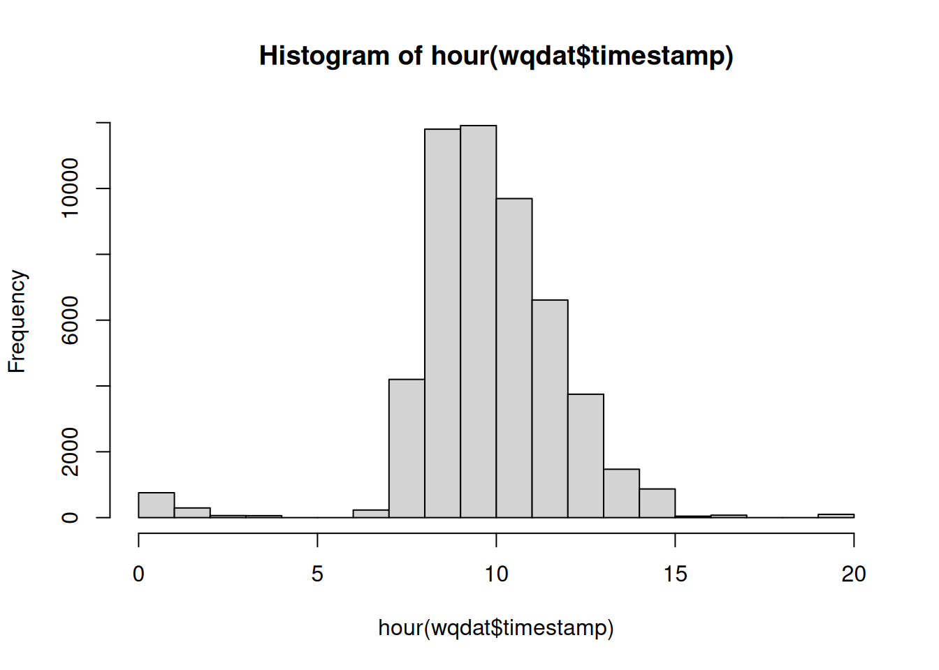
Below, we change the time zone attribute with force_tz. Note that the tzone argument is specified as "Etc/GMT+5", which is Eastern Time without daylight savings (see OlsonNames() for a list of acceptable time zones in R).
# convert to Eastern Time
wqdat <- mutate(wqdat, timestamp = force_tz(timestamp, tzone = "Etc/GMT+5"))

# verify new time zone
attr(wqdat$timestamp, "tzone")
[1] "Etc/GMT+5"Now we can create extra columns for different time components. This might be useful if we want to know what time of day most parameters are collected or if results vary seasonally (e.g., by month).
# create new columns for year, month, day, and hour
wqdat_dates <- mutate(wqdat,
  year = year(timestamp),
  month = month(timestamp),
  day = day(timestamp),
  hour = hour(timestamp)
)
head(wqdat_dates)
# A tibble: 6 × 11
station_no station_name parametertype_shortname parametertype_name
<dbl> <chr> <chr> <chr>
1 23113 Lake Panasoffkee 7 WQ_79 Alkalinity (CaCO3)
2 23113 Lake Panasoffkee 7 WQ_79 Alkalinity (CaCO3)
3 23113 Lake Panasoffkee 7 WQ_79 Alkalinity (CaCO3)
4 23113 Lake Panasoffkee 7 WQ_79 Alkalinity (CaCO3)
5 23113 Lake Panasoffkee 7 WQ_79 Alkalinity (CaCO3)
6 23113 Lake Panasoffkee 7 WQ_79 Alkalinity (CaCO3)
# ℹ 7 more variables: timestamp <dttm>, value <dbl>, unit_symbol <chr>,
# year <dbl>, month <dbl>, day <int>, hour <int>There are many more functions in dplyr, but you’ll use the ones above the most. As you can imagine, they are most effective when used together because there is never a single step in the data wrangling process. After the exercise, we’ll talk about how we can efficiently pipe functions to create a new data object.
2.6 Exercise 4
Now that you know the basic functions in dplyr and how to use them, let’s put them to use. Using wqdat, let’s select some columns of interest, filter by station, and rename one of the columns.
Import the water quality data file from your
datafolder usingread_csv()(load the tidyverse and here packages first if needed).Select the
timestamp,station_name,parametertype_name, andvaluecolumns. Assign this dataset to a new object in your workspace.Using the new object, filter to get all rows where Station is equal to
'Lake Panasoffkee 8'and parameter is equal toTemperature, Water(hint, filter by thestation_namecolumn andparametertype_name, don’t forget to use==).Convert the
timestampcolumn to the correct time zone (hint, usemutatewithforce_tzfor timezone"Etc/GMT+5").
Click to show/hide solution
library(tidyverse)
library(here)
wqdat <- read_csv(here('data', 'wqdat.csv'))
ex1 <- select(wqdat, timestamp, station_name, parametertype_name, value)
ex1 <- filter(ex1, station_name == "Lake Panasoffkee 8" & `parametertype_name` == "Temperature, Water")
ex1 <- mutate(ex1, timestamp = force_tz(timestamp, tzone = "Etc/GMT+5"))
2.7 Piping
A complete data wrangling exercise will always include multiple steps to go from the raw data to the output you need. Here’s a terrible wrangling example using functions from base R:
cropdat <- rawdat[1:28]
savecols <- data.frame(cropdat$Party, cropdat$`Last Inventory Year (2015)`)
names(savecols) <- c('Party','2015')
savecols$rank2015 <- rank(-savecols$`2015`)
top10df <- savecols[savecols$rank2015 <= 10,]
basedat <- cropdat[cropdat$Party %in% top10df$Party,]
Technically, if this works it’s not “wrong”, but there are a couple of issues that can cause problems. First, the flow of functions to manipulate the data is not obvious and this makes your code very hard to read. Second, lots of unnecessary intermediates have been created in your workspace. Anything that adds clutter should be avoided because R is fundamentally based on object assignments. The less you assign to variables in your environment the easier it will be to navigate complex scripts.
The good news is that you now know how to use the dplyr functions to wrangle data. The function names in dplyr were chosen specifically to be descriptive. This will make your code much more readable than if you were using base R counterparts. However, I haven’t told you how to easily link the functions. Fortunately, there’s an easy fix to this problem.
Recent versions of R provide a very useful method called piping that will make wrangling a whole lot easier. The idea is simple: a pipe (|>) is used to chain functions together. The output from one function becomes the input to the next function in the pipe. This avoids the need to create intermediate objects and creates a logical progression of steps that demystify the wrangling process.
Consider the simple example:
# not using pipes, select a column, filter rows
bad_ex <- select(wqdat, station_name, value)
bad_ex2 <- filter(bad_ex, value > 10)
With pipes, it looks like this:
# with pipes, select a column, filter rows
good_ex <- wqdat |>
  select(station_name, value) |>
  filter(value > 10)
Now we’ve created only one new object in our environment and we can clearly see that we select, then filter. The only real coding differences are the use of a pipe operator and now the select and filter functions only include the relevant information. You do not need to explicitly specify the data inputs in each function if you’re using piping. The pipe will always use the input that comes from above.
A couple comments about piping:
- It is very annoying to type the pipe operator. RStudio has a nice keyboard shortcut:
Crtl + Shift + Mfor Windows (useCmd + Shift + Mon a mac). Using it a few times will commit it to muscle memory. - It’s convention to start a new function on the next line after a pipe operator. This makes the code easier to read and you can also remove or comment out a single step in a long pipe.
- Don’t make your pipes too long, limit them to a particular data object or task.
2.8 Exercise 5
Now that we know how to pipe functions, let’s repeat exercise 4. You should already have code to select, filter, and mutate the data. Use the following to repeat the analysis but with pipes. You should only have to create one data object in this exercise.
Using your code from exercise four, try to replicate the steps using pipes. The steps we used in exercise four were:
From wqdat, select the
timestamp,station_name,parametertype_name, andvaluecolumnsFilter by
station_nameto get only station"Lake Panasoffkee 8"andparametertype_nameto get only"Temperature, Water"Correct the timezone for
timestampto"Etc/GMT+5"usingmutateandforce_tz.
Click to show/hide solution
ex2 <- wqdat |>
  select(timestamp, station_name, parametertype_name, value) |>
  filter(station_name == "Lake Panasoffkee 8" & `parametertype_name` == "Temperature, Water") |>
  mutate(timestamp = force_tz(timestamp, tzone = "Etc/GMT+5"))
head(ex2)
2.9 Next time
Now you should be able to answer (or be able to find answers to) the following:
- Why do we need to manipulate data?
- What is the tidyverse?
- What can you do with dplyr?
- What is piping?
Next we’ll continue with data wrangling.
2.10 Attribution
Content in this lesson was pillaged extensively from the USGS-R training curriculum here and R for Data Science.