Data wrangling part 1
Get the lesson R script: Data_Wrangling_1.R
Get the lesson data: download zip
Lesson Outline
Lesson Exercises
Goals
Data wrangling (manipulation, ninjery, cleaning, etc.) is the part of any data analysis that will take the most time. While it may not necessarily be fun, it is foundational to all the work that follows. I strongly believe that mastering these skills has more value than mastering a particular analysis. Check out this article if you don’t believe me.
We’ll have two hours to cover parts 1 and 2 of data wrangling. It’s an unrealistic expectation that you will be a ninja wrangler after this training. As such, the goals are to expose you to fundamentals and to develop an appreciation of what’s possible. I also want to provide resources that you can use for follow-up learning on your own.
After this lesson you should be able to answer (or be able to find answers to) the following:
- Why do we need to manipulate data?
- What is the tidyverse?
- What can you do with dplyr?
- What is piping?
The tidyverse
The tidyverse is a set of packages that work in harmony because they share common data representations and design. The tidyverse package is designed to make it easy to install and load core packages from the tidyverse in a single command. With tidyverse, you’ll be able to address all steps of data exploration.
From the excellent book, R for Data Science, data exploration is the art of looking at your data, rapidly generating hypotheses, quickly testing them, then repeating again and again and again. Tools in the tidyverse also have direct application to more formal analyses with many of the other available R packages on CRAN.
You should already have the tidyverse installed, but let’s give it a go if you haven’t done this part yet:
# install
install.packages('tidyverse')
After installation, we can load the package:
# load
library(tidyverse)
## -- Attaching packages --------------------------------------- tidyverse 1.3.0 --## v ggplot2 3.3.3 v purrr 0.3.4
## v tibble 3.1.0 v stringr 1.4.0
## v tidyr 1.1.3 v forcats 0.5.1
## v readr 1.4.0## -- Conflicts ------------------------------------------ tidyverse_conflicts() --
## x dplyr::filter() masks stats::filter()
## x dplyr::lag() masks stats::lag()Notice that the messages you get after loading are a bit different from other packages. That’s because tidyverse is a package that manages other packages. Loading tidyverse will load all of the core packagbes:
- ggplot2, for data visualisation.
- dplyr, for data manipulation.
- tidyr, for data tidying.
- readr, for data import.
- purrr, for functional programming.
- tibble, for tibbles, a modern re-imagining of data frames.
Other packages (e.g., readxl) are also included but you will probably not use these as frequently.
A nice feature of tidyverse is the ability to check for and install new versions of each package:
tidyverse_update()
#> The following packages are out of date:
#>  * broom (0.4.0 -> 0.4.1)
#>  * DBI   (0.4.1 -> 0.5)
#>  * Rcpp  (0.12.6 -> 0.12.7)
#> Update now?
#>
#> 1: Yes
#> 2: No
As you’ll soon learn using R, there are often several ways to achieve the same goal. The tidyverse provides tools to address problems that can be solved with other packages or even functions from the base installation. Tidyverse is admittedly an opinionated approach to data exploration, but it’s popularity and rapid growth within the R community is a testament to the power of the tools that are provided.
Data wrangling with dplyr
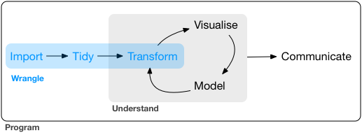
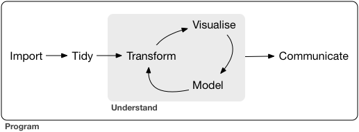
The data wrangling process includes data import, tidying, and transformation. The process directly feeds into, and is not mutually exclusive, with the understanding or modelling side of data exploration. More generally, I consider data wrangling as the manipulation or combination of datasets for the purpose of analysis.
Wrangling begins with import and ends with an output of some kind, such as a plot or a model, but is more often a dataset that has been altered from a raw dataset to suit the needs of an analysis. In a perfect world, the wrangling process is linear with no need for back-tracking. In reality, we often uncover more information about a dataset, either through wrangling or modeling, that warrants re-evaluation or even gathering more data. Data also come in many forms and the form you need for analysis is rarely the required form of the input data. For these reasons, data wrangling will consume most of your time in data exploration.
All wrangling is based on a purpose. No one wrangles for the sake of wrangling (usually), so the process always begins by answering the following two questions:
- What do my input data look like?
- What should my input data look like given what I want to do?
At the most basic level, going from what your data looks like to what it should look like will require a few key operations. Some common examples:
- Selecting specific variables
- Filtering observations by some criteria
- Adding or modifying existing variables
- Renaming variables
- Arranging rows by a variable
- Summarizing variable conditional on others
The dplyr package provides easy tools for these common data manipulation tasks. It is built to work directly with data frames and this is one of the foundational packages in what is now known as the tidyverse. The philosophy of dplyr is that one function does one thing and the name of the function says what it does. This is where the tidyverse generally departs from other packages and even base R. It is meant to be easy, logical, and intuitive. There is a lot of great info on dplyr. If you have an interest, I’d encourage you to look more. The vignettes are particularly good.
I’ll demonstrate the examples with the fishdat dataset from the last lesson. This dataset includes over 30000 catch records of fish from Old Tampa Bay.
# import the data
fishdat <- read_csv('data/fishdat.csv')

# see first six rows
head(fishdat)
## # A tibble: 6 x 12
## OBJECTID Reference Sampling_Date yr Gear ExDate Bluefish
## <dbl> <chr> <date> <dbl> <dbl> <dttm> <dbl>
## 1 1550020 TBM1996032006 1996-03-20 1996 300 2018-04-12 10:27:38 0
## 2 1550749 TBM1996032004 1996-03-20 1996 22 2018-04-12 10:25:23 0
## 3 1550750 TBM1996032004 1996-03-20 1996 22 2018-04-12 10:25:23 0
## 4 1550762 TBM1996032207 1996-03-22 1996 20 2018-04-12 10:25:23 0
## 5 1550828 TBM1996042601 1996-04-26 1996 160 2018-04-12 10:25:23 0
## 6 1550838 TBM1996051312 1996-05-13 1996 300 2018-04-12 10:25:23 0
## # ... with 5 more variables: Common Snook <dbl>, Mullets <dbl>, Pinfish <dbl>,
## # Red Drum <dbl>, Sand Seatrout <dbl># dimensions
dim(fishdat)## [1] 2844 12# column names
names(fishdat)## [1] "OBJECTID" "Reference" "Sampling_Date" "yr"
## [5] "Gear" "ExDate" "Bluefish" "Common Snook"
## [9] "Mullets" "Pinfish" "Red Drum" "Sand Seatrout"# structure
str(fishdat)## spec_tbl_df[,12] [2,844 x 12] (S3: spec_tbl_df/tbl_df/tbl/data.frame)
## $ OBJECTID : num [1:2844] 1550020 1550749 1550750 1550762 1550828 ...
## $ Reference : chr [1:2844] "TBM1996032006" "TBM1996032004" "TBM1996032004" "TBM1996032207" ...
## $ Sampling_Date: Date[1:2844], format: "1996-03-20" "1996-03-20" ...
## $ yr : num [1:2844] 1996 1996 1996 1996 1996 ...
## $ Gear : num [1:2844] 300 22 22 20 160 300 300 300 300 22 ...
## $ ExDate : POSIXct[1:2844], format: "2018-04-12 10:27:38" "2018-04-12 10:25:23" ...
## $ Bluefish : num [1:2844] 0 0 0 0 0 0 0 0 0 0 ...
## $ Common Snook : num [1:2844] 0 0 0 0 0 0 0 0 0 0 ...
## $ Mullets : num [1:2844] 0 0 0 0 0 0 0 0 0 0 ...
## $ Pinfish : num [1:2844] 0 54 0 80 0 0 0 0 1 1 ...
## $ Red Drum : num [1:2844] 0 0 1 0 4 0 0 0 0 0 ...
## $ Sand Seatrout: num [1:2844] 1 0 0 0 0 1 5 66 0 0 ...
## - attr(*, "spec")=
## .. cols(
## .. OBJECTID = col_double(),
## .. Reference = col_character(),
## .. Sampling_Date = col_date(format = ""),
## .. yr = col_double(),
## .. Gear = col_double(),
## .. ExDate = col_datetime(format = ""),
## .. Bluefish = col_double(),
## .. `Common Snook` = col_double(),
## .. Mullets = col_double(),
## .. Pinfish = col_double(),
## .. `Red Drum` = col_double(),
## .. `Sand Seatrout` = col_double()
## .. )Selecting
Let’s begin using dplyr. Don’t forget to load the tidyverse if you haven’t done so already. We can use the select function to, you guessed it, select columns.
# first, select some columns
dplyr_sel1 <- select(fishdat, Sampling_Date, Gear, Pinfish)
head(dplyr_sel1)
## # A tibble: 6 x 3
## Sampling_Date Gear Pinfish
## <date> <dbl> <dbl>
## 1 1996-03-20 300 0
## 2 1996-03-20 22 54
## 3 1996-03-20 22 0
## 4 1996-03-22 20 80
## 5 1996-04-26 160 0
## 6 1996-05-13 300 0# select everything but ObjectId and ExDate
dplyr_sel2 <- select(fishdat, -OBJECTID, -ExDate)
head(dplyr_sel2)## # A tibble: 6 x 10
## Reference Sampling_Date yr Gear Bluefish `Common Snook` Mullets Pinfish
## <chr> <date> <dbl> <dbl> <dbl> <dbl> <dbl> <dbl>
## 1 TBM19960320~ 1996-03-20 1996 300 0 0 0 0
## 2 TBM19960320~ 1996-03-20 1996 22 0 0 0 54
## 3 TBM19960320~ 1996-03-20 1996 22 0 0 0 0
## 4 TBM19960322~ 1996-03-22 1996 20 0 0 0 80
## 5 TBM19960426~ 1996-04-26 1996 160 0 0 0 0
## 6 TBM19960513~ 1996-05-13 1996 300 0 0 0 0
## # ... with 2 more variables: Red Drum <dbl>, Sand Seatrout <dbl># select columns that contain the letter c
dplyr_sel3 <- select(fishdat, matches('c'))
head(dplyr_sel3)## # A tibble: 6 x 3
## OBJECTID Reference `Common Snook`
## <dbl> <chr> <dbl>
## 1 1550020 TBM1996032006 0
## 2 1550749 TBM1996032004 0
## 3 1550750 TBM1996032004 0
## 4 1550762 TBM1996032207 0
## 5 1550828 TBM1996042601 0
## 6 1550838 TBM1996051312 0Filtering
After selecting columns, you’ll probably want to remove observations that don’t fit some criteria. For example, maybe you want to remove all rows with low catch or maybe you want to look only at fish caught in Gear 20 (a 21 m seine net).
# now filter observations with more than 30 Pinfish caught
dplyr_high_catch <- filter(fishdat, Pinfish > 30)
head(dplyr_high_catch)
## # A tibble: 6 x 12
## OBJECTID Reference Sampling_Date yr Gear ExDate Bluefish
## <dbl> <chr> <date> <dbl> <dbl> <dttm> <dbl>
## 1 1550749 TBM1996032004 1996-03-20 1996 22 2018-04-12 10:25:23 0
## 2 1550762 TBM1996032207 1996-03-22 1996 20 2018-04-12 10:25:23 0
## 3 1555103 TBM1996022010 1996-02-20 1996 22 2018-04-12 10:25:29 0
## 4 1572931 TBM1996080603 1996-08-06 1996 160 2018-04-12 10:25:36 0
## 5 1572932 TBM1996080604 1996-08-06 1996 160 2018-04-12 10:25:36 0
## 6 1573079 TBM1996062104 1996-06-21 1996 20 2018-04-12 10:26:15 0
## # ... with 5 more variables: Common Snook <dbl>, Mullets <dbl>, Pinfish <dbl>,
## # Red Drum <dbl>, Sand Seatrout <dbl># now filter observations for Gear type as 20
dplyr_gear20 <- filter(fishdat, Gear == 20)
head(dplyr_gear20)## # A tibble: 6 x 12
## OBJECTID Reference Sampling_Date yr Gear ExDate Bluefish
## <dbl> <chr> <date> <dbl> <dbl> <dttm> <dbl>
## 1 1550762 TBM1996032207 1996-03-22 1996 20 2018-04-12 10:25:23 0
## 2 1555259 TBM1996022104 1996-02-21 1996 20 2018-04-12 10:25:31 0
## 3 1573079 TBM1996062104 1996-06-21 1996 20 2018-04-12 10:26:15 0
## 4 1576651 TBM1996022007 1996-02-20 1996 20 2018-04-12 10:25:24 0
## 5 1584465 TBM1996061917 1996-06-19 1996 20 2018-04-12 10:26:04 0
## 6 1584803 TBM1996011905 1996-01-19 1996 20 2018-04-12 10:25:26 0
## # ... with 5 more variables: Common Snook <dbl>, Mullets <dbl>, Pinfish <dbl>,
## # Red Drum <dbl>, Sand Seatrout <dbl>Filtering can take a bit of time to master because there are several ways to tell R what you want. Within the filter function, the working part is a logical selection of TRUE and FALSE values that are used to select rows (TRUE means I want that row, FALSE means I don’t). Every selection within the filter function, no matter how complicated, will always be a T/F vector. This is similar to running queries on a database if you’re familiar with SQL.
To use filtering effectively, you have to know how to select the observations that you want using the comparison operators. R provides the standard suite: >, >=, <, <=, != (not equal), and == (equal). When you’re starting out with R, the easiest mistake to make is to use = instead of == when testing for equality.
Multiple arguments to filter() are combined with “and”: every expression must be true in order for a row to be included in the output. For other types of combinations, you’ll need to use Boolean operators yourself: & is “and”, | is “or”, and ! is “not”. This is the complete set of Boolean operations.
![]()
Let’s start combining filtering operations.
# get rows with > 30 and less than 100 Pinfish
filt1 <- filter(fishdat, Pinfish > 30 & Pinfish < 100)
head(filt1)
## # A tibble: 6 x 12
## OBJECTID Reference Sampling_Date yr Gear ExDate Bluefish
## <dbl> <chr> <date> <dbl> <dbl> <dttm> <dbl>
## 1 1550749 TBM1996032004 1996-03-20 1996 22 2018-04-12 10:25:23 0
## 2 1550762 TBM1996032207 1996-03-22 1996 20 2018-04-12 10:25:23 0
## 3 1555103 TBM1996022010 1996-02-20 1996 22 2018-04-12 10:25:29 0
## 4 1572931 TBM1996080603 1996-08-06 1996 160 2018-04-12 10:25:36 0
## 5 1573079 TBM1996062104 1996-06-21 1996 20 2018-04-12 10:26:15 0
## 6 1635253 TBM1997031016 1997-03-10 1997 20 2018-04-12 10:29:33 0
## # ... with 5 more variables: Common Snook <dbl>, Mullets <dbl>, Pinfish <dbl>,
## # Red Drum <dbl>, Sand Seatrout <dbl># get rows with gear type 20 or red drum larger than 40
filt2 <- filter(fishdat, Gear == 20 | `Red Drum` > 40)
head(filt2)## # A tibble: 6 x 12
## OBJECTID Reference Sampling_Date yr Gear ExDate Bluefish
## <dbl> <chr> <date> <dbl> <dbl> <dttm> <dbl>
## 1 1550762 TBM1996032207 1996-03-22 1996 20 2018-04-12 10:25:23 0
## 2 1555259 TBM1996022104 1996-02-21 1996 20 2018-04-12 10:25:31 0
## 3 1573079 TBM1996062104 1996-06-21 1996 20 2018-04-12 10:26:15 0
## 4 1576651 TBM1996022007 1996-02-20 1996 20 2018-04-12 10:25:24 0
## 5 1584465 TBM1996061917 1996-06-19 1996 20 2018-04-12 10:26:04 0
## 6 1584803 TBM1996011905 1996-01-19 1996 20 2018-04-12 10:25:26 0
## # ... with 5 more variables: Common Snook <dbl>, Mullets <dbl>, Pinfish <dbl>,
## # Red Drum <dbl>, Sand Seatrout <dbl># get rows gear 20 or gear 5
filt3 <- filter(fishdat, Gear == 20 | Gear == 5)
head(filt3)## # A tibble: 6 x 12
## OBJECTID Reference Sampling_Date yr Gear ExDate Bluefish
## <dbl> <chr> <date> <dbl> <dbl> <dttm> <dbl>
## 1 1550762 TBM1996032207 1996-03-22 1996 20 2018-04-12 10:25:23 0
## 2 1555259 TBM1996022104 1996-02-21 1996 20 2018-04-12 10:25:31 0
## 3 1573079 TBM1996062104 1996-06-21 1996 20 2018-04-12 10:26:15 0
## 4 1576651 TBM1996022007 1996-02-20 1996 20 2018-04-12 10:25:24 0
## 5 1584465 TBM1996061917 1996-06-19 1996 20 2018-04-12 10:26:04 0
## 6 1584803 TBM1996011905 1996-01-19 1996 20 2018-04-12 10:25:26 0
## # ... with 5 more variables: Common Snook <dbl>, Mullets <dbl>, Pinfish <dbl>,
## # Red Drum <dbl>, Sand Seatrout <dbl># get rows with gear 20 or gear 5 using different syntax
filt4 <- filter(fishdat, Gear %in% c(20, 5))
head(filt4)## # A tibble: 6 x 12
## OBJECTID Reference Sampling_Date yr Gear ExDate Bluefish
## <dbl> <chr> <date> <dbl> <dbl> <dttm> <dbl>
## 1 1550762 TBM1996032207 1996-03-22 1996 20 2018-04-12 10:25:23 0
## 2 1555259 TBM1996022104 1996-02-21 1996 20 2018-04-12 10:25:31 0
## 3 1573079 TBM1996062104 1996-06-21 1996 20 2018-04-12 10:26:15 0
## 4 1576651 TBM1996022007 1996-02-20 1996 20 2018-04-12 10:25:24 0
## 5 1584465 TBM1996061917 1996-06-19 1996 20 2018-04-12 10:26:04 0
## 6 1584803 TBM1996011905 1996-01-19 1996 20 2018-04-12 10:25:26 0
## # ... with 5 more variables: Common Snook <dbl>, Mullets <dbl>, Pinfish <dbl>,
## # Red Drum <dbl>, Sand Seatrout <dbl>As a side note, any variable (i.e., column name) with spaces or non-standard characters can be referenced by enclosing it with backticks (see here).
Mutating
Now that we’ve seen how to filter observations and select columns of a data frame, maybe we want to add a new column. In dplyr, mutate allows us to add new columns. These can be vectors you are adding or based on expressions applied to existing columns. For instance, we have a column for average size in mm and maybe we want to convert to cm.
# add a column as bluefish divided by 100
dplyr_mut <- mutate(fishdat, Bluefish_p100 = Bluefish / 100)
head(dplyr_mut)
## # A tibble: 6 x 13
## OBJECTID Reference Sampling_Date yr Gear ExDate Bluefish
## <dbl> <chr> <date> <dbl> <dbl> <dttm> <dbl>
## 1 1550020 TBM1996032006 1996-03-20 1996 300 2018-04-12 10:27:38 0
## 2 1550749 TBM1996032004 1996-03-20 1996 22 2018-04-12 10:25:23 0
## 3 1550750 TBM1996032004 1996-03-20 1996 22 2018-04-12 10:25:23 0
## 4 1550762 TBM1996032207 1996-03-22 1996 20 2018-04-12 10:25:23 0
## 5 1550828 TBM1996042601 1996-04-26 1996 160 2018-04-12 10:25:23 0
## 6 1550838 TBM1996051312 1996-05-13 1996 300 2018-04-12 10:25:23 0
## # ... with 6 more variables: Common Snook <dbl>, Mullets <dbl>, Pinfish <dbl>,
## # Red Drum <dbl>, Sand Seatrout <dbl>, Bluefish_p100 <dbl># add a column for many/few mullet
dplyr_mut2 <- mutate(fishdat, mullet_cat = ifelse(Mullets < 20, 'few', 'many'))
head(dplyr_mut2)## # A tibble: 6 x 13
## OBJECTID Reference Sampling_Date yr Gear ExDate Bluefish
## <dbl> <chr> <date> <dbl> <dbl> <dttm> <dbl>
## 1 1550020 TBM1996032006 1996-03-20 1996 300 2018-04-12 10:27:38 0
## 2 1550749 TBM1996032004 1996-03-20 1996 22 2018-04-12 10:25:23 0
## 3 1550750 TBM1996032004 1996-03-20 1996 22 2018-04-12 10:25:23 0
## 4 1550762 TBM1996032207 1996-03-22 1996 20 2018-04-12 10:25:23 0
## 5 1550828 TBM1996042601 1996-04-26 1996 160 2018-04-12 10:25:23 0
## 6 1550838 TBM1996051312 1996-05-13 1996 300 2018-04-12 10:25:23 0
## # ... with 6 more variables: Common Snook <dbl>, Mullets <dbl>, Pinfish <dbl>,
## # Red Drum <dbl>, Sand Seatrout <dbl>, mullet_cat <chr>Some other useful dplyr functions include arrange to sort the observations (rows) by a column and rename to (you guessed it) rename a column.
# arrange by maximum size
dplyr_arr <- arrange(fishdat, `Sand Seatrout`)
head(dplyr_arr)
## # A tibble: 6 x 12
## OBJECTID Reference Sampling_Date yr Gear ExDate Bluefish
## <dbl> <chr> <date> <dbl> <dbl> <dttm> <dbl>
## 1 1550749 TBM1996032004 1996-03-20 1996 22 2018-04-12 10:25:23 0
## 2 1550750 TBM1996032004 1996-03-20 1996 22 2018-04-12 10:25:23 0
## 3 1550762 TBM1996032207 1996-03-22 1996 20 2018-04-12 10:25:23 0
## 4 1550828 TBM1996042601 1996-04-26 1996 160 2018-04-12 10:25:23 0
## 5 1551311 TBM1996032209 1996-03-22 1996 300 2018-04-12 10:25:20 0
## 6 1551335 TBM1996041807 1996-04-18 1996 22 2018-04-12 10:25:24 0
## # ... with 5 more variables: Common Snook <dbl>, Mullets <dbl>, Pinfish <dbl>,
## # Red Drum <dbl>, Sand Seatrout <dbl># rename some columns
dplyr_rnm <- rename(fishdat, snook = `Common Snook`)
head(dplyr_rnm)## # A tibble: 6 x 12
## OBJECTID Reference Sampling_Date yr Gear ExDate Bluefish
## <dbl> <chr> <date> <dbl> <dbl> <dttm> <dbl>
## 1 1550020 TBM1996032006 1996-03-20 1996 300 2018-04-12 10:27:38 0
## 2 1550749 TBM1996032004 1996-03-20 1996 22 2018-04-12 10:25:23 0
## 3 1550750 TBM1996032004 1996-03-20 1996 22 2018-04-12 10:25:23 0
## 4 1550762 TBM1996032207 1996-03-22 1996 20 2018-04-12 10:25:23 0
## 5 1550828 TBM1996042601 1996-04-26 1996 160 2018-04-12 10:25:23 0
## 6 1550838 TBM1996051312 1996-05-13 1996 300 2018-04-12 10:25:23 0
## # ... with 5 more variables: snook <dbl>, Mullets <dbl>, Pinfish <dbl>,
## # Red Drum <dbl>, Sand Seatrout <dbl>There are many more functions in dplyr but the ones above are by far the most used. As you can imagine, they are most effective when used together because there is never only one step in the data wrangling process. After the exercise, we’ll talk about how we can efficiently pipe the functions in dplyr to create a new data object.
Exercise 4
Now that you know the basic functions in dplyr and how to use them, let’s put them to use. Using fishdat, let’s select some columns of interest, filter by gear type, and rename one of the columns.
Select the
Reference,Sampling_Date,Gear, andSand Seatroutcolumns. Assign this dataset to a new object in your workspace. Don’t forget to use backticks to select column names that have spaces.Using the new object, filter to get all rows where Gear is equal to 20 (hint, filter by the
Gearcolumn and don’t forget ot use==).Rename the
Sampling_Datecolumn todate.
ex1 <- select(fishdat, Reference, Sampling_Date, Gear, `Sand Seatrout`)
ex1 <- filter(ex1, Gear == 20)
ex1 <- rename(ex1, date = Sampling_Date)
nrow(ex1)
Piping
A complete data wrangling exercise will always include multiple steps to go from the raw data to the output you need. Here’s a terrible wrangling example using functions from base R:
cropdat <- rawdat[1:28]
savecols <- data.frame(cropdat$Party, cropdat$`Last Inventory Year (2015)`)
names(savecols) <- c('Party','2015')
savecols$rank2015 <- rank(-savecols$`2015`)
top10df <- savecols[savecols$rank2015 <= 10,]
basedat <- cropdat[cropdat$Party %in% top10df$Party,]
Technically, if this works it’s not “wrong”, but there are a couple of issues that can lead to problems down the line. First, the flow of functions to manipulate the data is not obvious and this makes your code very hard to read. Second, lots of unecessary intermediates have been created in your workspace. Anything that adds to clutter should be avoided because R is fundamentally based on object assignments. The less you assign as a variable in your environment the easier it will be to navigate complex scripts.
The good news is that you now know how to use the dplyr functions to wrangle data. The function names in dplyr were chosen specifically to be descriptive. This will make your code much more readable than if you were using base R counterparts. The bad news is that I haven’t told you how to easily link the functions. Fortunately, there’s an easy fix to this problem.
The magrittr package (comes with tidyverse) provides a very useful method called piping that will make wrangling a whole lot easier. The idea is simple: a pipe (%>%) is used to chain functions together. The output from one function becomes the input to the next function in the pipe. This avoids the need to create intermediate objects and creates a logical progression of steps that demystify the wrangling process.
Consider the simple example:
# not using pipes, select a column, filter rows
bad_ex <- select(fishdat, Gear, `Common Snook`)
bad_ex2 <- filter(bad_ex, `Common Snook` > 25)
With pipes, it looks like this:
# with pipes, select a column, filter rows
good_ex <- fishdat %>%
  select(Gear, `Common Snook`) %>%
  filter(`Common Snook` > 25)
Now we’ve created only one new object in our environment and we can clearly see that we select, then filter. The only real coding difference is now the select and filter functions only include the relevant information. You do not need to specify a data object as input to a function if you’re using piping. The pipe will always use the input that comes from above.
A couple comments about piping:
- I find it very annoying to type the pipe operator (six key strokes!). RStudio has a nice keyboard shortcut:
Crtl + Shift + Mfor Windows (useCmd + Shift + Mon a mac). - It’s convention to start a new function on the next line after a pipe operator. This makes the code easier to read and you can also comment out a single step in a long pipe.
- Don’t make your pipes too long, limit them to a particular data object or task.
Exercise 5
Now that we know how to pipe functions, let’s repeat exercise 4. You should already have code to select and filter the data. Use the following to repeat the analysis but with pipes. You should only have to create one data object in this exercise.
- Using your code from exercise four, try to replicate the steps using pipes. The steps we used in exercise four were:
- From fishdat, select the
Reference,Sampling_Date,Gear, andSand Seatroutcolumns - Filter by
Gearto get only gear 20 - Rename
Sampling_Datetodate
- From fishdat, select the
ex2 <- fishdat %>%
  select(Reference, Sampling_Date, Gear, `Sand Seatrout`) %>%
  filter(Gear == 20) %>%
  rename(date = Sampling_Date)
head(ex2)
Next time
Now you should be able to answer (or be able to find answers to) the following:
- Why do we need to manipulate data?
- What is the tidyverse?
- What can you do with dplyr?
- What is piping?
Next we’ll continue with data wrangling.
Attribution
Content in this lesson was pillaged extensively from the USGS-R training curriculum here and R for data Science.