Creating an R package crash course
This document provides a step-by-step guide to creating a simple R package. It is not meant as a comprehensive list of resources about package development, but instead is meant to serve as an archive of steps outlined in the live demo. There are many, many resources online that can help you build R packages and we encourage you to look elsewhere for a more detailed coverage of packages. See the Resources at the end of this document.
The workflow in this document also begins by creating a GitHub repository, which of course assumes you have a GitHub account. Linking a repository to an R package can also occur at any step in the package development process, although it should begin at the start for full version control.
This document also uses a simple processing script and dataset as examples for creating the package. You can download them and follow along in this document to create your own package. The approach is meant to demonstrate a common challenge most analysts or researchers may have where a script has been written to accomplish some task, but it may be nice to “package” the code into discrete functions for easy access.
Outline
Step 1
Start by creating a new repository on your GitHub account. On your main page, click repositories on the top, then New. You should see a screen like this:
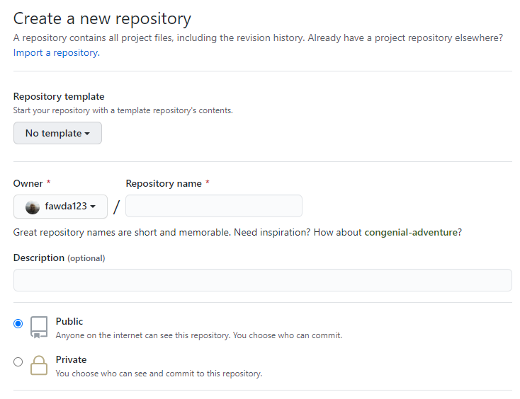
Give the repository a name and a brief description of what you plan to include. After you create the repository, you should see a screen with information about setting up the repository on your local machine.
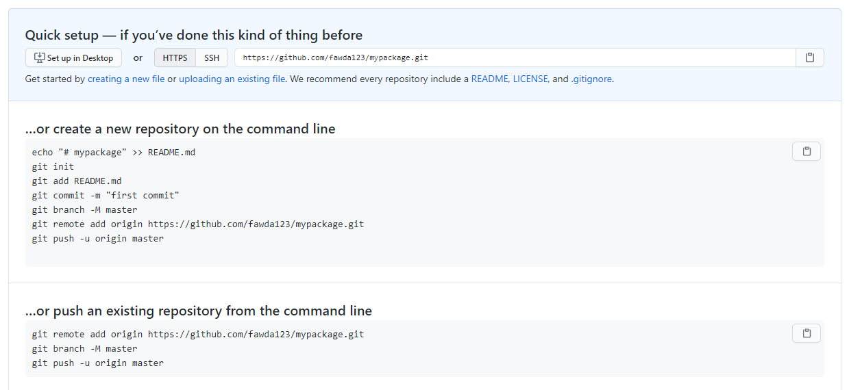
These instructions tell you how to setup a repository on the command line. In the next step, we’ll do this directly in RStudio.
Step 2
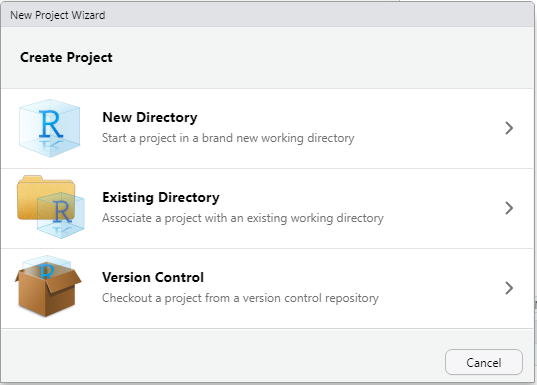
In RStudio, go to the File Menu and select New Project.... Select the version control option when the new project dialogue box pops up.
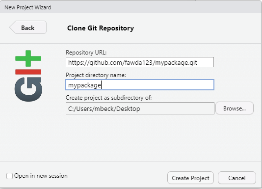
Select the Git option and then enter the URL for your Github repository. The URL can be copied to your clipboard from the repository webpage you just setup. Make sure it ends in .git.
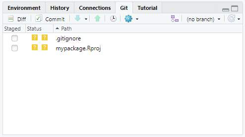
The RStudio project will open in a new R session after you enter the repository information. It will only include two files, the .gitignore file and the .Rproj file that is included in every RStudio project. The former can be used to add files you don’t want to track on version control.
Now that the project is created, you can make your first commit and push it to your repository. Click the “Commit” button under the Git pane in RStudio.
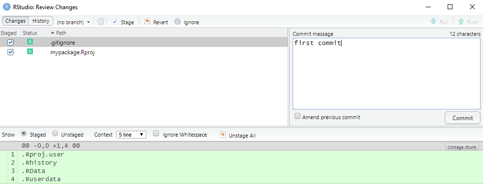
A new window will popup with the files that you want to push to GitHub. Click the box next to each file to stage them, enter a commit message, and push them to GitHub. The push button is the green arrow.
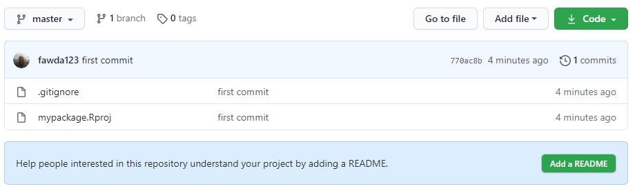
Your repository page on GitHub will now include the files you committed and pushed.
Step 3
We can start populating our RStudio project with R code and data now that the project is setup and under full version control with Git. Copy the data processing script and data into the project home directory. This is a script that imports the Tampa Bay fisheries data, summarizes length data for a selected species and gear type, then creates a plot of the result.
# load packages
library(tidyverse)
library(gridExtra)
library(patchwork)

# load data
tbhdat <- read.csv('data/example_len_dat.csv', stringsAsFactors = F)

# preprocess length data
Plot <- tbhdat %>%
  filter(Scientificname == 'Lagodon rhomboides') %>%
  ggplot() +
  geom_histogram(aes(x=sl), color = "black", fill = NA, binwidth = 10) +
  labs(x = "Standard length (mm)", y = "Frequency") +
  facet_wrap(~ Gear, ncol = 1) +
  theme_classic() +
  theme(panel.border = element_rect(color = "black", fill = NA)) +
  theme(strip.background = element_rect(fill = "gray90"))

#get length summary data
summary <- tbhdat %>%
  filter(Scientificname == 'Lagodon rhomboides') %>%
  group_by(Gear) %>%
  summarise(min_sl = min(sl),
            max_sl = max(sl),
            mean_sl = round(mean(sl), digits = 2),
            sd_sl = round(sd(sl), digits = 2),
            Num_lengths = n()) %>%
  ungroup()

# combine plot and summary table
Plot / gridExtra::tableGrob(summary, rows = NULL) +
  plot_layout(heights = c(2,0.8)) +
  plot_annotation(title = 'Lagodon rhomboides', theme= theme(plot.title = element_text(face = "italic")))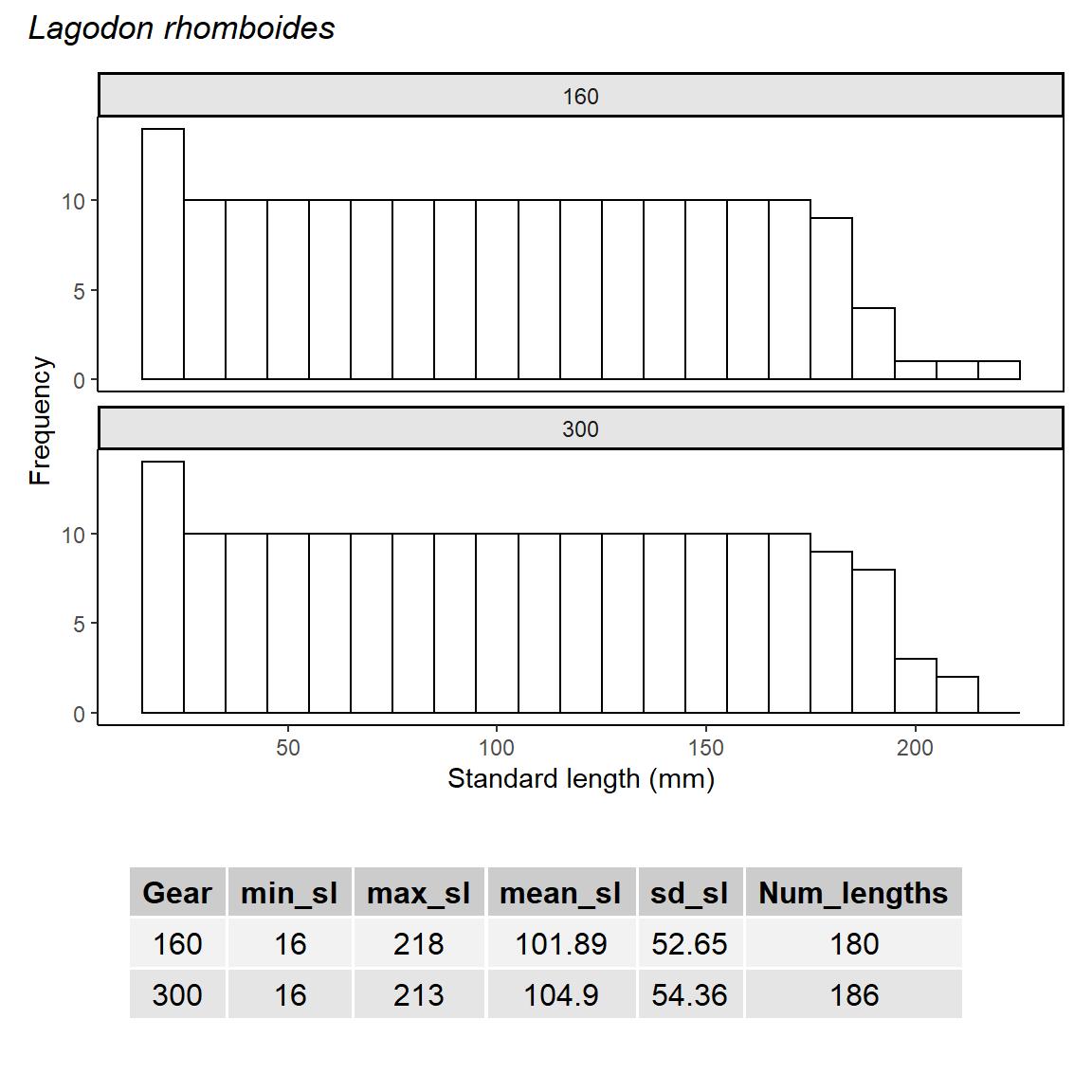
It’s likely we’ll want to create these plots for different species. We can create a function that simplifies this for us so we don’t have to rerun the script every time to create the new plot. Highlight the lines of code that process and plot the data, then use the Extract function shortcut in RStudio (Ctrl + Alt + x). You should see something like this. This will get you most of the way and with some minor editing we can create a new function.
sumplot <- function(tbhdat, Scientificname){

  # preprocess length data
  Plot <- tbhdat %>%
    filter(Scientificname == !!Scientificname) %>%
    ggplot() +
    geom_histogram(aes(x=sl), color = "black", fill = NA, binwidth = 10) +
    labs(x = "Standard length (mm)", y = "Frequency") +
    facet_wrap(~ Gear, ncol = 1) +
    theme_classic() +
    theme(panel.border = element_rect(color = "black", fill = NA)) +
    theme(strip.background = element_rect(fill = "gray90"))

  #get length summary data
  summary <- tbhdat %>%
    filter(Scientificname == !!Scientificname) %>%
    group_by(Gear) %>%
    summarise(min_sl = min(sl),
              max_sl = max(sl),
              mean_sl = round(mean(sl), digits = 2),
              sd_sl = round(sd(sl), digits = 2),
              Num_lengths = n()) %>%
    ungroup()

  # combine plot and summary table
  p <- Plot / gridExtra::tableGrob(summary, rows = NULL) +
    plot_layout(heights = c(2,0.8)) +
    plot_annotation(title = Scientificname, theme= theme(plot.title = element_text(face = "italic")))

  return(p)

}
Now save this function to a separate R script called sumplot.R and put it in a folder called R in the project’s home directory. You can simplify the original processing script by sourcing the new script with source().
# load packages
library(tidyverse)
library(gridExtra)
library(patchwork)

source('R/sumplot.R')

# load data
tbhdat <- read.csv('data/example_len_dat.csv', stringsAsFactors = F)

sumplot(tbhdat, 'Lagodon rhomboides')
Step 4
Create the package template in your project using the create_package() function from the usethis package.
usethis::create_package()Follow the on-screen instructions and select the option to overwrite the .Rproj file. You should now see your project similar as before but with a new file tree structure. This is the basic template for an R package.
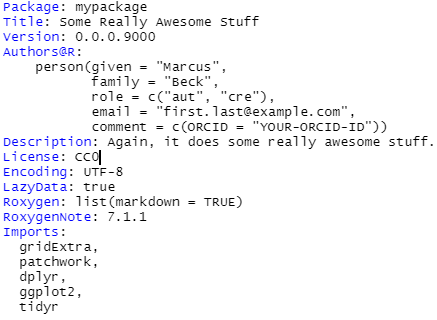
The first thing to do is to modify the DESCRIPTION file. This is metadata for your package and also includes the other packages that your package depends on. It should look something like this when you’re done. Note the Imports field where we import dplyr, tidyr, ggplot2, gridExtra, and patchwork packages that are used in our plotting function. Note that our original script imported the tidyverse which includes dplyr, ggplot2, and tidyr. It is not possible to include the tidyverse directly in the Imports field because it is a collection of multiple packages.
Step 5
After the DESCRIPTION file is done, you can start creating documentation for your functions. This uses the roxygen2 packages that comes with RStudio to convert the text documentation in the .R function file to a .Rd file in the man folder. This is all done automatically in a later step.
Open the R function file you created in Step 3. Place the cursor anywhere inside the function and use the “Insert Roxygen Skeleton” shortcut with Ctrl + Shift + Alt + r. You should see this at the top of your function.
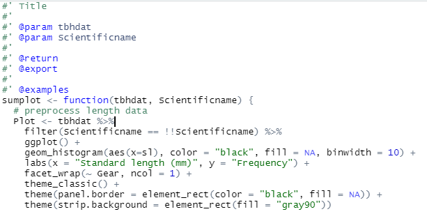
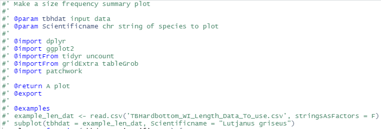
Enter any relevant information in the roxygen documentation to describe your function. You must also include an @import field to explicitly include any packages that have functions used within your function. It should look something like this when you’re done.
Finally, the documentation .Rd file is created with the document() function from devtools. You’ll see a new man folder after running the function.
devtools::document()Step 6
If you’re satisfied with your package, you can load it with load_all() to test the functions. This loads your package in your current Environment as if it was a package you loaded with the library() function, where the only difference is the package is not actually installed on your computer.
devtools::load_all()You can also run checks on your package to make sure you’ve done everything right, i.e., all dependencies are correctly indicated, the examples run, the documentation is correct, etc. This is always a good idea to make sure that you and others can actually install and use the package. These are the same checks used by CRAN for incoming packages.
devtools::check()Step 7
Push your final package to GitHub using the same workflow as before (i.e., stage, commit, and push all changes). After this is done, you or anybody else can download and install your package.
devtools::install_github('fawda123/mypackage')