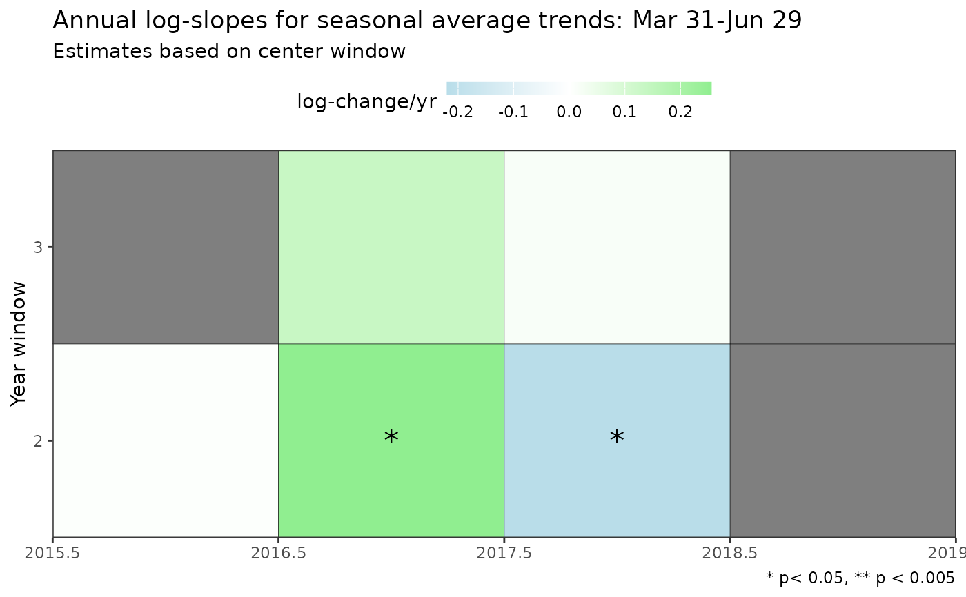
Plot seasonal rates of change based on average estimates for multiple window widths

Usage

show_sumtrndseason(
  mod,
  doystr = 1,
  doyend = 364,
  yromit = NULL,
  justify = c("center", "left", "right"),
  win = 5:15,
  txtsz = 6,
  cols = c("lightblue", "lightgreen"),
  base_size = 11
)

Arguments

mod: input model object as returned by anlz_gam
doystr: numeric indicating start Julian day for extracting averages
doyend: numeric indicating ending Julian day for extracting averages
yromit: optional numeric vector for years to omit from the plot, see details
justify: chr string indicating the justification for the trend window
win: numeric vector indicating number of years to use for the trend window
txtsz: numeric for size of text labels inside the plot
cols: vector of low/high colors for trends
base_size: numeric indicating base font size, passed to theme_bw

Value

A ggplot2 plot

Details

This function plots output from anlz_sumtrndseason.

The optional yromit vector can be used to omit years from the plot and trend assessment. This may be preferred if seasonal estimates for a given year have very wide confidence intervals likely due to limited data, which can skew the trend assessments.

Examples

library(dplyr)

# data to model
tomod <- rawdat %>%
  filter(station %in% 34) %>%
  filter(param %in% 'chl') %>% 
  filter(yr > 2015)

mod <- anlz_gam(tomod, trans = 'log10')
show_sumtrndseason(mod, doystr = 90, doyend = 180, justify = 'center', win = 2:3)