This package can be used to assess water quality trends for long-term monitoring data in estuaries using Generalized Additive Models and mixed-effects meta-analysis (Wood 2017; Sera et al. 2019). These models are appropriate for data typically from surface water quality monitoring programs at roughly monthly or biweekly collection intervals, covering at least a decade of observations (e.g., Cloern and Schraga 2016). Daily or continuous monitoring data covering many years are not appropriate for these methods, due to computational limitations and a goal of the analysis to estimate long-term, continuous trends from irregular or discontinuous sampling.
Basic usage
The sample dataset rawdat is included in the package and
is used for the examples below. This dataset includes monthly time
series data over ~30 years for nine stations in South Bay, San Francisco
Estuary. Data are available for 4 water quality parameters. All data are
in long format with one observation per row.
The data are pre-processed to work with the GAM fitting functions
included in this package. The columns include date, station number,
parameter name, and value for the date. Additional date columns are
included that describe the day of year (doy), date in
decimal time (cont_year), year (yr), and month
(mo as character label). These are required for model
fitting or use with the analysis/plotting functions.
head(rawdat)#> date station param value doy cont_year yr mo
#> 1 1990-02-27 18 chl 1.0333333 58 1990.156 1990 Feb
#> 2 1990-04-18 18 chl 1.6333333 108 1990.293 1990 Apr
#> 3 1990-05-30 18 chl 1.6000000 150 1990.408 1990 May
#> 4 1990-07-30 18 chl 5.2333333 211 1990.575 1990 Jul
#> 5 1990-12-06 18 chl 0.9333333 340 1990.929 1990 Dec
#> 6 1991-02-06 18 chl 1.6333333 37 1991.099 1991 FebOne GAM model can be fit to the time series data. Each GAM fits
additive smoothing functions to describe variation of the response
variable (value) over time, where time is measured as a
continuous number. The basic GAM used by this package is as follows:
-
S: value ~ s(year, k = large)
The cont_year vector is measured as a continuous numeric
variable for the annual effect (e.g., January 1st, 2000 is 2000.0, July
1st, 2000 is 2000.5, etc.). The function s() models
cont_year as a smoothed, non-linear variable. The optimal
amount of smoothing on cont_year is determined by
cross-validation as implemented in the mgcv package (Wood 2017) and an upper theoretical upper limit
on the number of knots for k should be large enough to
allow sufficient flexibility in the smoothing term. The upper limit of
k was chosen as 12 times the number of years for the input
data. If insufficient data are available to fit a model with the
specified k, the number of knots is decreased until the
data can be modelled, e.g., 11 times the number of years, 10 times the
number of years, etc.
The anlz_gam() function is used to fit the model. First,
the raw data are filtered to select only station 34 and the chlorophyll
parameter. The model is fit using a log-10 transformation of the
response variable. Available transformation options are log-10
(log10) or identity (ident). The log-10
transformation is used by default if not specified by the user.
tomod <- rawdat %>%
 filter(station %in% 34) %>%
 filter(param %in% "chl")
mod <- anlz_gam(tomod, trans = "log10")
mod
#>
#> Family: gaussian
#> Link function: identity
#>
#> Formula:
#> value ~ s(cont_year, k = 348)
#>
#> Estimated degrees of freedom:
#> 219 total = 219.93
#>
#> GCV score: 0.07280572All remaining functions use the model results to assess fit, calculate seasonal metrics and trends, and plot results.
The fit can be assessed using anlz_smooth() and
anlz_fit(), where the former assesses the individual
smoother functions and the latter assesses overall fit. The
anlz_smooth() results show the results for the fit to the
cont_year smoother as the effective degrees of freedom
(edf), the reference degrees of freedom
(Ref.df), the test statistic (F), and
statistical significance (p-value). The significance is in
part based on the difference between edf and
Ref.df. The anlz_fit() results show the
overall summary of the model as Akaike Information Criterion
(AIC), the generalized cross-validation score
(GCV), and the R2 values. Lower values for
AIC and GCV and higher values for
R2 indicate better model fit.
anlz_smooth(mod)#> smoother edf Ref.df F p.value
#> 1 s(cont_year) 218.9304 262.4482 4.788546 0
anlz_fit(mod)#> AIC GCV R2
#> GCV.Cp -3.16688 0.07280572 0.6842621The plotting functions show the results in different formats. If appropriate for the response variable, the model predictions are back-transformed and the scales on each plot are shown in log10-scale to preserve the values of the results.
The show_prddoy() function shows estimated results by
day of year with separate lines for each year.
ylab <- "Chlorophyll-a"
show_prddoy(mod, ylab = ylab)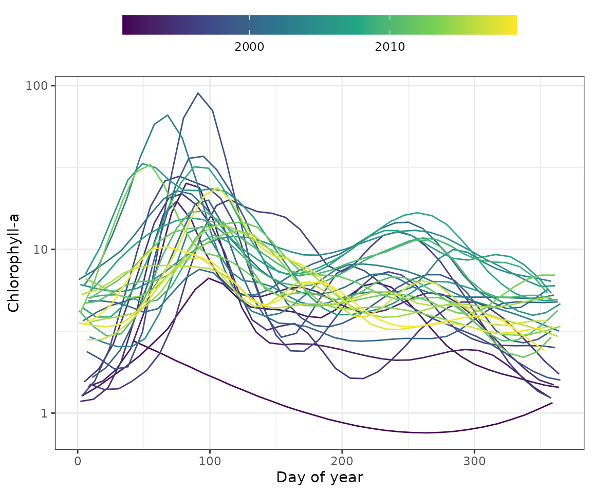
The show_prdseries() function shows predictions for the
model across the entire time series. Points are the observed data and
the lines are the predicted.
show_prdseries(mod, ylab = ylab)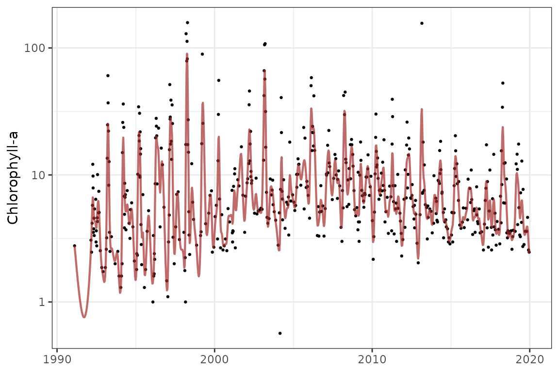
The show_prdseason() function is similar except that the
model predictions are grouped by month. This provides a simple visual
depiction of changes by month over time. The trend analysis functions
below can be used to statistically test the seasonal changes.
show_prdseason(mod, ylab = ylab)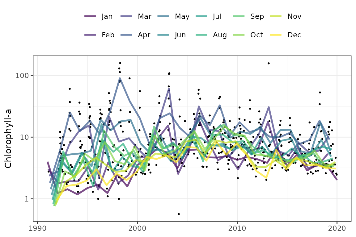
Finally, the show_prd3d() function shows a
three-dimensional fit of the estimated trends across year and day of
year with the z-axis showing the estimates for the response
variable.
show_prd3d(mod, ylab = ylab)Trend testing
Statistical tests for evaluating trends are available in this package. These methods are considered “secondary” analyses that use results from a fitted GAM to evaluate trends or changes over time. In particular, significance of changes over time are evaluated using mixed-effect meta-analysis (Sera et al. 2019) applied to the GAM results to allow for full propagation of uncertainty between methods. Each test includes a plotting method to view the results.
Evaluating changes between time periods
The anlz_perchg() and show_perchg()
functions can be used to compare annual averages between two time
periods of interest. The functions require base and test year inputs
that are used for comparison. More than one year can be entered for the
base and test years, e.g., baseyr = c(1990, 1992, 1993)
vs. testyr = c(2014, 2015, 2016).
anlz_perchg(mod, baseyr = 2006, testyr = 2017)#> # A tibble: 1 × 4
#> baseval testval perchg pval
#> <dbl> <dbl> <dbl> <dbl>
#> 1 9.78 5.35 -45.3 0.000376To plot the results for one GAM, use the show_perchg()
function. The plot title summarizes the results.
show_perchg(mod, baseyr = 2006, testyr = 2017, ylab = "Chlorophyll-a (ug/L)")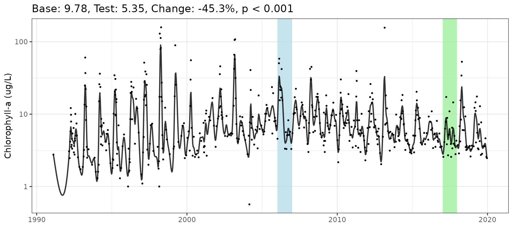
Evaluating seasonal changes over time
The anlz_metseason(), anlz_mixmeta(), and
show_metseason() functions evaluate seasonal metrics (e.g.,
mean, max, etc.) between years, including an assessment of the trend for
selected years using mixed-effects meta-analysis modelling. These
functions require inputs for the seasonal ranges to evaluate
(doyend, doystr) and years for assessing the
trend in the seasonal averages/metrics (yrstr,
yrend).
The anlz_metseason() function estimates the seasonal
metrics (including uncertainty as standard error) for results from the
GAM fit. The seasonal metric can be any summary function available in R,
such as seasonal maxima (max), minima (min),
variance (var), or others. The function uses repeated
resampling of the GAM model coefficients to simulate multiple time
series as an estimate of uncertainty for the summary parameter.
The inputs for anlz_metseason() include the seasonal
range as day of year using start (doystr) and end
(doyend) days and the metfun and
nsim arguments to specify the summary function and number
of simulations, respectively. Here we show the estimate for the maximum
chlorophyll in each season, using a relatively low number of
simulations. Repeating this function will produce similar but slightly
different results because the estimates are stochastic. In practice, a
large value for nsim should be used to produce accurate
results (e.g., nsim = 1e5).
metseason <- anlz_metseason(mod, metfun = max, doystr = 90, doyend = 180, nsim = 100)
metseason
#> # A tibble: 29 × 7
#> yr met se bt_lwr bt_upr bt_met dispersion
#> <dbl> <dbl> <dbl> <dbl> <dbl> <dbl> <dbl>
#> 1 1991 0.264 0.426 0.301 14.1 2.06 0.0434
#> 2 1992 0.825 0.0676 5.52 10.2 7.49 0.0434
#> 3 1993 1.41 0.102 18.1 45.5 28.7 0.0434
#> 4 1994 1.12 0.0900 9.76 22.0 14.6 0.0434
#> 5 1995 1.27 0.0845 14.4 30.8 21.0 0.0434
#> 6 1996 1.31 0.108 13.9 37.0 22.7 0.0434
#> 7 1997 1.41 0.0998 18.2 44.9 28.6 0.0434
#> 8 1998 1.96 0.104 63.3 162. 101. 0.0434
#> 9 1999 1.58 0.138 22.8 79.4 42.5 0.0434
#> 10 2000 1.32 0.122 13.4 40.3 23.3 0.0434
#> # ℹ 19 more rowsThe anlz_mixmeta() function uses results from the
anlz_metseason() to estimate the trend in the seasonal
metric over a selected year range. Here, we evaluate the seasonal trend
from 2006 to 2017 for the seasonal estimate of the model results
above.
anlz_mixmeta(metseason, yrstr = 2006, yrend = 2017)#> Call: mixmeta::mixmeta(formula = met ~ yr, S = S, data = totrnd, random = ~1 |
#> yr, method = "reml")
#>
#> Fixed-effects coefficients:
#> (Intercept) yr
#> 69.0965 -0.0338
#>
#> 12 units, 1 outcome, 12 observations, 2 fixed and 1 random-effects parameters
#> logLik AIC BIC
#> 8.3047 -10.6094 -9.7017The show_metseason() function plots the seasonal metrics
and trends over time. The anlz_metseason() and
anlz_mixmeta() functions are used internally to get the
predictions. The same arguments for these functions are used for
show_metseason, with the mean as the default metric.
show_metseason(mod, doystr = 90, doyend = 180, yrstr = 2006, yrend = 2017, ylab = "Chlorophyll-a (ug/L)")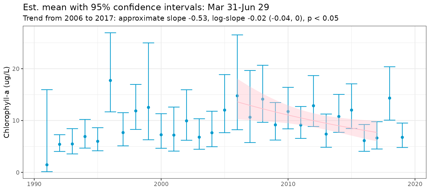
To plot only the seasonal metrics, the regression line showing trends
over time can be suppressed by setting one or both of yrstr
and yrend as NULL.
show_metseason(mod, doystr = 90, doyend = 180, yrstr = NULL, yrend = NULL, ylab = "Chlorophyll-a (ug/L)")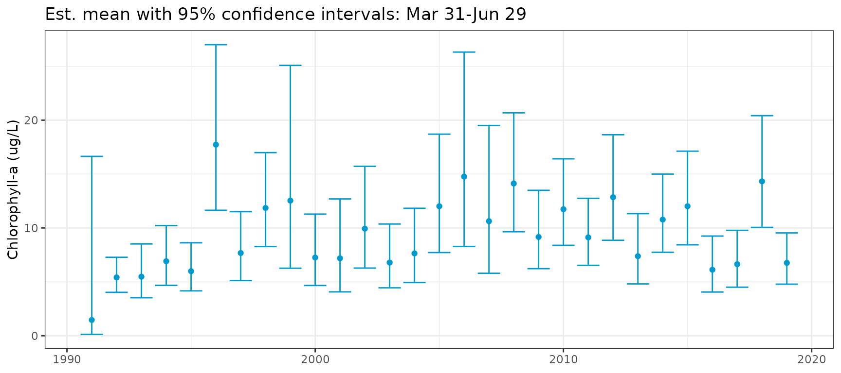
Adding an argument for metfun to
show_metseason() will plot results and trends for a metric
other than the average. Note the use of nsim in this
example. In practice, a much higher value should be used (e.g.,
nsim = 1e5)
show_metseason(mod, metfun = max, nsim = 100, doystr = 90, doyend = 180, yrstr = 2006, yrend = 2017, ylab = "Chlorophyll-a (ug/L)")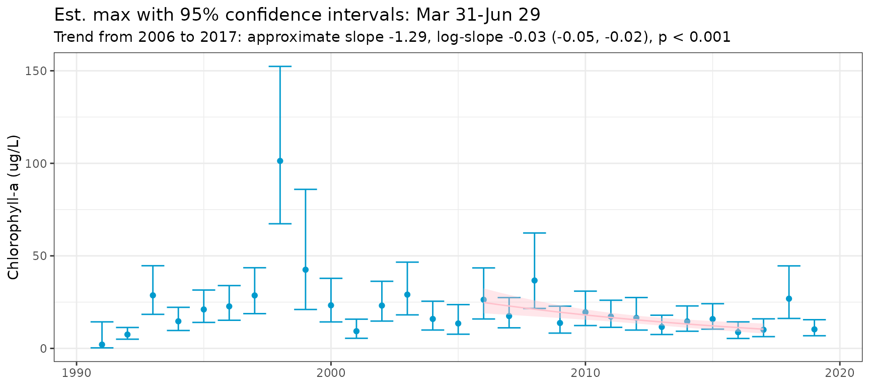
For convenience, the anlz_sumstats() function returns a
list of summary statistics for the GAM and associated mixed-effect
meta-analysis model. This function can be useful for creating tabular
results of the models. The list output includes mixmet as a
mixmeta object of the fitted mixed-effects meta-analysis
trend model, metseason as a tibble object of the fitted
seasonal metrics as returned by anlz_metseason() or
anlz_avgseason(), summary of the
mixmet object, and coeffs as a tibble object
of the slope estimate coefficients from mixmet. An
approximately linear slope estimate will be included as
slope.approx in coeffs if
trans = 'log10' for the GAM used in mod.
anlz_sumstats(mod, metfun = mean, doystr = 90, doyend = 180, yrstr = 2006, yrend = 2017)#> $mixmet
#> Call: mixmeta::mixmeta(formula = met ~ yr, S = S, data = totrnd, random = ~1 |
#> yr, method = "reml")
#>
#> Fixed-effects coefficients:
#> (Intercept) yr
#> 46.4015 -0.0226
#>
#> 12 units, 1 outcome, 12 observations, 2 fixed and 1 random-effects parameters
#> logLik AIC BIC
#> 8.6916 -11.3831 -10.4754
#>
#>
#> $metseason
#> # A tibble: 29 × 7
#> yr met se bt_lwr bt_upr bt_met dispersion
#> <dbl> <dbl> <dbl> <dbl> <dbl> <dbl> <dbl>
#> 1 1991 0.115 0.529 0.134 15.9 1.46 0.0434
#> 2 1992 0.684 0.0649 4.04 7.26 5.41 0.0434
#> 3 1993 0.689 0.0956 3.56 8.43 5.48 0.0434
#> 4 1994 0.790 0.0866 4.68 10.2 6.91 0.0434
#> 5 1995 0.728 0.0814 4.15 8.65 5.99 0.0434
#> 6 1996 1.20 0.0922 11.7 26.9 17.7 0.0434
#> 7 1997 0.835 0.0899 5.12 11.5 7.68 0.0434
#> 8 1998 1.02 0.0815 8.21 17.1 11.9 0.0434
#> 9 1999 1.05 0.154 6.26 25.1 12.5 0.0434
#> 10 2000 0.811 0.0975 4.67 11.3 7.25 0.0434
#> # ℹ 19 more rows
#>
#> $summary
#> Call: mixmeta::mixmeta(formula = met ~ yr, S = S, data = totrnd, random = ~1 |
#> yr, method = "reml")
#>
#> Univariate extended random-effects meta-regression
#> Dimension: 1
#> Estimation method: REML
#>
#> Fixed-effects coefficients
#> Estimate Std. Error z Pr(>|z|) 95%ci.lb 95%ci.ub
#> (Intercept) 46.4015 18.6384 2.4896 0.0128 9.8708 82.9321 *
#> yr -0.0226 0.0093 -2.4385 0.0147 -0.0407 -0.0044 *
#> ---
#> Signif. codes: 0 '***' 0.001 '**' 0.01 '*' 0.05 '.' 0.1 ' ' 1
#>
#> Random-effects (co)variance components
#> Formula: ~1 | yr
#> Structure: General positive-definite
#> Std. Dev
#> 0.0533
#>
#> Univariate Cochran Q-test for residual heterogeneity:
#> Q = 13.3901 (df = 10), p-value = 0.2027
#> I-square statistic = 25.3%
#>
#> 12 units, 1 outcome, 12 observations, 2 fixed and 1 random-effects parameters
#> logLik AIC BIC
#> 8.6916 -11.3831 -10.4754
#>
#>
#> $coeffs
#> # A tibble: 1 × 8
#> slope.approx slope slope.se z p likelihood ci.lb ci.ub
#> <dbl> <dbl> <dbl> <dbl> <dbl> <dbl> <dbl> <dbl>
#> 1 -0.537 -0.0226 0.00926 -2.44 0.0147 0.993 -0.0407 -0.00443The seasonal estimates and mixed-effects meta-analysis regression can
be used to estimate the rate of seasonal change across the time series.
For any given year and seasonal metric, a trend can be estimated within
a specific window (i.e., yrstr and yrend
arguments in show_metseason()). This trend can be estimated
for every year in the period of record to estimate the rate of change
over time for the seasonal estimates.
The anlz_trndseason() function estimates the rate of
change and the show_trndseason() function plots the
results. For both, all inputs required for the
anlz_metseason() function are required, in addition to the
desired window width to evaluate for each year (win) and
the justification for the window as "left",
"right", or "center" from each year
(justify).
It’s important to note the behavior of the centering for window
widths (win argument) if choosing even or odd values. For
left and right windows, the exact number of years in win is
used. For example, a left-centered window for 1990 of ten years will
include exactly ten years from 1990, 1991, … , 1999. The same applies to
a right-centered window, e.g., for 1990 it would include 1981, 1982, …,
1990 (if those years have data). However, for a centered window, picking
an even number of years for the window width will create a slightly
off-centered window because it is impossible to center on an even number
of years. For example, if win = 8 and
justify = 'center', the estimate for 2000 will be centered
on 1997 to 2004 (three years left, four years right, eight years total).
Centering for window widths with an odd number of years will always
create a symmetrical window, i.e., if win = 7 and
justify = 'center', the estimate for 2000 will be centered
on 1997 and 2003 (three years left, three years right, seven years
total).
trndseason <- anlz_trndseason(mod, doystr = 90, doyend = 180, justify = 'left', win = 5)
head(trndseason)
#> # A tibble: 6 × 12
#> yr met se bt_lwr bt_upr bt_met dispersion yrcoef pval appr_yrcoef
#> <dbl> <dbl> <dbl> <dbl> <dbl> <dbl> <dbl> <dbl> <dbl> <dbl>
#> 1 1991 0.115 0.532 0.132 16.1 1.46 0.0434 0.0273 0.403 0.360
#> 2 1992 0.684 0.0653 4.03 7.27 5.41 0.0434 0.103 0.0381 1.80
#> 3 1993 0.689 0.0969 3.54 8.48 5.48 0.0434 0.0700 0.265 1.29
#> 4 1994 0.790 0.0867 4.67 10.2 6.91 0.0434 0.0582 0.341 1.24
#> 5 1995 0.728 0.0806 4.16 8.62 5.99 0.0434 0.0488 0.466 1.18
#> 6 1996 1.20 0.0907 11.8 26.7 17.7 0.0434 -0.0613 0.213 -1.51
#> # ℹ 2 more variables: yrcoef_lwr <dbl>, yrcoef_upr <dbl>The show_trndseason() function can be used to plot the
results directly, one model at a time.
show_trndseason(mod, doystr = 90, doyend = 180, justify = 'left', win = 5, ylab = 'Chl. change/yr, average')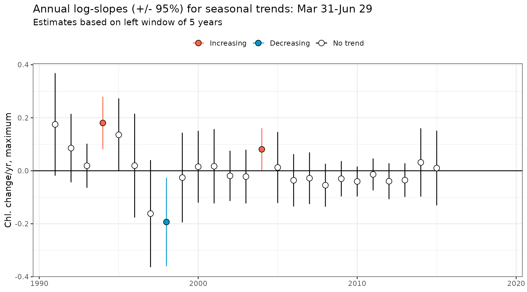
As before, adding an argument for metfun to
show_trndseason() will plot results and trends for a metric
other than the average. Note the use of nsim in this
example. In practice, a much higher value should be used (e.g.,
nsim = 1e5)
show_trndseason(mod, metfun = max, nsim = 100, doystr = 90, doyend = 180, justify = 'left', win = 5, ylab = 'Chl. change/yr, maximum')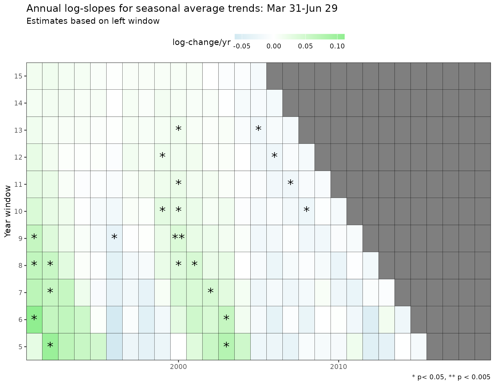
The results supplied by show_trndseason() can be
extended to multiple window widths by stacking the results into a single
plot. Below, results for window widths from 5 to 15 years are shown
using the show_sumtrndseason() function for a selected
seasonal range using a left-justified window. This function only works
with average seasonal metrics due to long processing times with other
metrics. To retrieve the results in tabular form, use
anlz_sumtrndseason().
show_sumtrndseason(mod, doystr = 90, doyend = 180, justify = 'left', win = 5:15)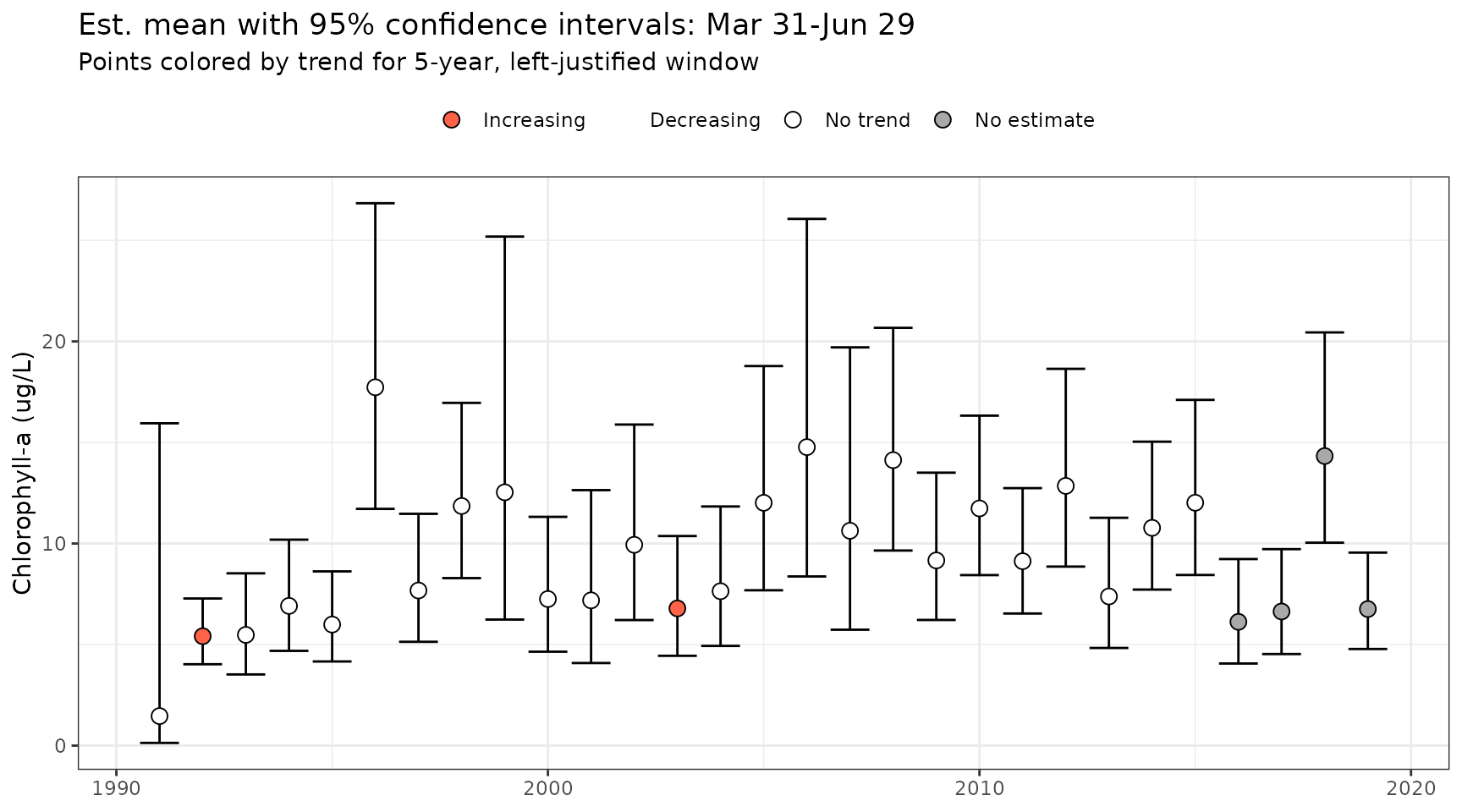
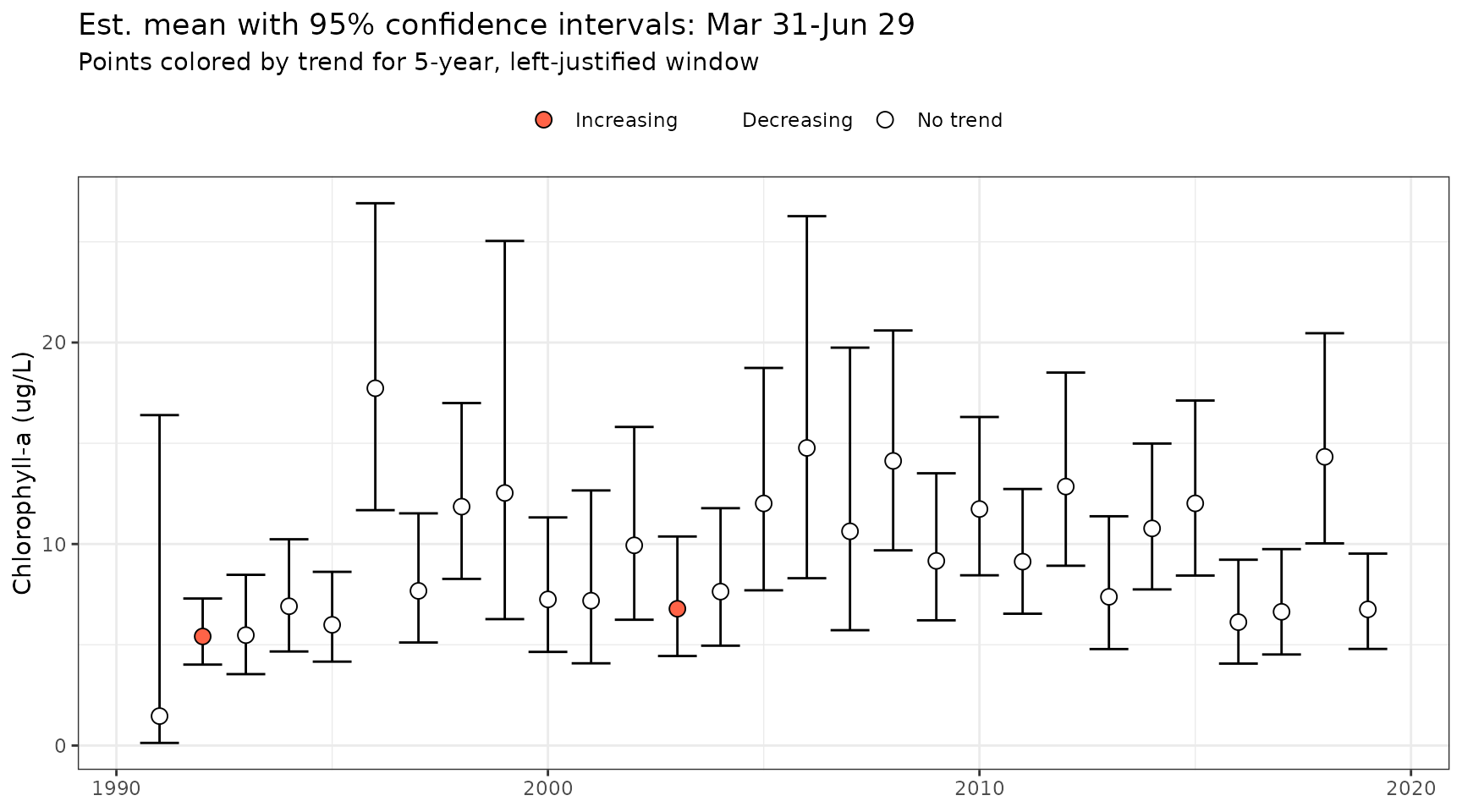
Lastly, the plots returned by show_metseason() and
show_trndseason() can be combined using the
show_mettrndseason() function. This plot will show the
seasonal metrics from the GAM as in show_metseason() with
the colors of the points for the seasonal metrics colored by the
significance of the moving window trends shown in
show_trndseason(). The four colors indicate increasing,
decreasing, no trend, or no estimate (i.e., too few points for the
window). Most of the arguments for show_metseason() and
show_trndseason() apply to
show_mettrndseason().
show_mettrndseason(mod, metfun = mean, doystr = 90, doyend = 180, ylab = "Chlorophyll-a (ug/L)", win = 5, justify = 'left')
Four colors are used to define increasing, decreasing, no trend, or
no estimate. The cmbn argument can be used to combine the
no trend and no estimate colors into one color and label. Although this
may be desired for aesthetic reasons, the colors and labels may be
misleading with the default names since no trend is shown for points
where no estimates were made.
show_mettrndseason(mod, metfun = mean, doystr = 90, doyend = 180, ylab = "Chlorophyll-a (ug/L)", win = 5, justify = 'left', cmbn = T)