# install
install.packages('tidyverse')3 Data wrangling part 2
Get the lesson R script: data_wrangling_2.R
Get the lesson data: download zip
3.1 Lesson Outline
3.2 Lesson Exercises
3.3 Goals
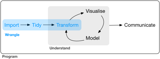
In this lesson we’ll continue our discussion of data wrangling with the tidyverse. Data wrangling is the manipulation or combination of datasets for the purpose of understanding. It fits within the broader scheme of data exploration, described as the art of looking at your data, rapidly generating hypotheses, quickly testing them, then repeating again and again and again (from R for Data Science, 2nd Ed., as is most of today’s content).
Always remember that wrangling is based on a purpose. The process always begins by answering the following two questions:
- What do my input data look like?
- What should my input data look like given what I want to do?
You define what steps to take to get your data from input to where you want to go.
Last lesson we learned the following functions from the dplyr package (cheatsheet here):
- Selecting variables with
select - Filtering observations by some criteria with
filter - Adding or modifying existing variables with
mutate - Arranging rows by a variable with
arrange - Renaming variables with
rename
As before, we only have one hour to cover the basics of data wrangling. It’s an unrealistic expectation that you will be a ninja wrangler after this training. As such, the goals are to expose you to fundamentals and to develop an appreciation of what’s possible. I also want to provide resources that you can use for follow-up learning on your own.
After this lesson you should be able to answer (or be able to find answers to) the following:
- How are data joined?
- What is tidy data?
- How do I summarize a dataset?
You should already have the tidyverse package installed, but let’s give it a go if you haven’t done this part yet:
After installation, we can load the package:
library(tidyverse)── Attaching core tidyverse packages ──────────────────────── tidyverse 2.0.0 ──
✔ dplyr 1.1.4 ✔ readr 2.1.5
✔ forcats 1.0.1 ✔ stringr 1.6.0
✔ ggplot2 4.0.0 ✔ tibble 3.3.0
✔ lubridate 1.9.4 ✔ tidyr 1.3.1
✔ purrr 1.2.0
── Conflicts ────────────────────────────────────────── tidyverse_conflicts() ──
✖ dplyr::filter() masks stats::filter()
✖ dplyr::lag() masks stats::lag()
ℹ Use the conflicted package (<http://conflicted.r-lib.org/>) to force all conflicts to become errors3.4 Combining data
Combining data is a common task of data wrangling. Perhaps we want to combine information between two datasets that share a common identifier. As a real world example, our fisheries data contain information about fish catch, but we also want to include spatial information about the stations (i.e., lat, lon). We would need to (and we will) combine data if this information is in two different places. Combining data with dplyr is called joining.
All joins require that each of the tables can be linked by shared identifiers. These are called ‘keys’ and are usually represented as a separate column that acts as a unique variable for the observations. The “Station ID” is our common key, but remember that a key might need to be unique for each row. It doesn’t make sense to join two tables by station ID if multiple site visits were made. In that case, your keys should include some information about the site visit and station ID. In other words, you would need to join with two variables.
3.4.1 Types of joins
The challenge with joins is that the two datasets may not represent the same observations for a given key. For example, you might have one table with all observations for every key, another with only some observations, or two tables with only a few shared keys. What you get back from a join will depend on what’s shared between tables, in addition to the type of join you use.
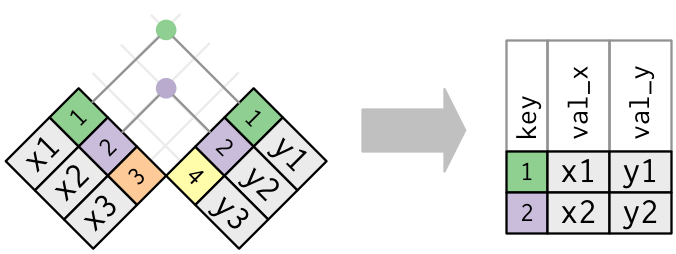
We can demonstrate types of joins with simple graphics. The first is an inner-join.
The second is an outer-join, and comes in three flavors: left, right, and full.
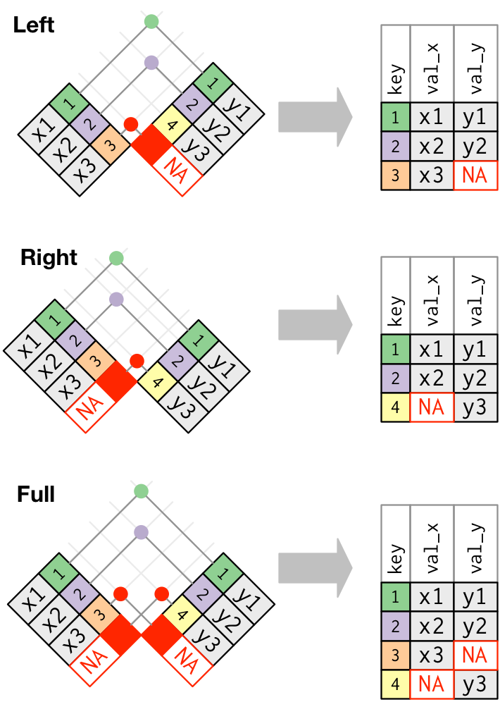
If all keys are shared between two data objects, then left, right, and full joins will give you the same result. I typically only use left_join just because it’s intuitive to me. This assumes that there is never any more information in the second table - it has the same or less keys as the original table.
The data we downloaded for this workshop included fisheries catch data and the locations of each station. If we want to plot any of the catch data by location, we need to join the two datasets.
# load the fish data
fishdat <- read_csv('data/fishdat.csv')

# load the station data
statloc <- read_csv('data/statloc.csv')

# join the two
joindat <- left_join(fishdat, statloc, by = 'Reference')
head(joindat)
# A tibble: 6 × 14
OBJECTID Reference Sampling_Date yr Gear ExDate Bluefish
<dbl> <chr> <date> <dbl> <dbl> <dttm> <dbl>
1 1550020 TBM1996032006 1996-03-20 1996 300 2018-04-12 10:27:38 0
2 1550749 TBM1996032004 1996-03-20 1996 22 2018-04-12 10:25:23 0
3 1550750 TBM1996032004 1996-03-20 1996 22 2018-04-12 10:25:23 0
4 1550762 TBM1996032207 1996-03-22 1996 20 2018-04-12 10:25:23 0
5 1550828 TBM1996042601 1996-04-26 1996 160 2018-04-12 10:25:23 0
6 1550838 TBM1996051312 1996-05-13 1996 300 2018-04-12 10:25:23 0
# ℹ 7 more variables: `Common Snook` <dbl>, Mullets <dbl>, Pinfish <dbl>,
# `Red Drum` <dbl>, `Sand Seatrout` <dbl>, Latitude <dbl>, Longitude <dbl>A final note about joins is that you will have relationships between two tables defined as one-to-one, one-to-many, many-to-one, or many-to-many. Ofen times you may expect a one-to-one join (i.e., one row in table x will always correspond to one row in table y), but another relationship is observed (e.g., one row in table x corresponds to more than one row in table y, a one-to-many join). The join functions in dplyr will notify you if this occurs depending on the type of join you use. This is good because it tells you how to interpret the results of the join and whether or not you may have unexpected results. In general, you should have a prior expectation of the relationship between two tables. You can be explicit with the type of relationship you expect by including the arguments relationship = 'one-to-one' (or other types) in your join function.
3.5 Exercise 6
For this exercise we’ll repeat the join we just did, but on a subset of the data. We’re going to select some columns of interest from our fisheries dataset, filter by gear type, then use full_join() with the station data. Try to use pipes if you can.
Select the
Reference,Sampling_Date,Gear, andCommon Snookcolumns from the fisheries dataset (hint, useselectfrom dplyr).Filter the fisheries dataset by gear type 20 (hint, use
filter == 20). Check the dimensions of the new dataset withdim.Use a
full_jointo join the fisheries dataset with the station location dataset. What is the key value for joining?Check the dimensions of the new table. What happened?
Click to show/hide solution
# load the fish data
fishdat <- read_csv('data/fishdat.csv')

# load the station data
statloc <- read_csv('data/statloc.csv')

# wrangle before join
joindat <- fishdat |>
  select(Reference, Sampling_Date, Gear, `Common Snook`) |>
  filter(Gear == 20)

dim(joindat)

# full join
joindat <- joindat |>
  full_join(statloc, by = 'Reference')

dim(joindat)
3.6 Tidy data
The opposite of a tidy dataset is a messy dataset. You should always work towards a tidy data set as an outcome of the wrangling process. Tidy data are easy to work with and will make downstream analysis much simpler. This will become apparent when we start summarizing and plotting our data.
To help understand tidy data, it’s useful to look at alternative ways of representing data. The example below shows the same data organised in four different ways. Each dataset shows the same values of four variables country, year, population, and cases, but each dataset organises the values differently. Only one of these examples is tidy.
table1# A tibble: 6 × 4
country year cases population
<chr> <dbl> <dbl> <dbl>
1 Afghanistan 1999 745 19987071
2 Afghanistan 2000 2666 20595360
3 Brazil 1999 37737 172006362
4 Brazil 2000 80488 174504898
5 China 1999 212258 1272915272
6 China 2000 213766 1280428583table2# A tibble: 12 × 4
country year type count
<chr> <dbl> <chr> <dbl>
1 Afghanistan 1999 cases 745
2 Afghanistan 1999 population 19987071
3 Afghanistan 2000 cases 2666
4 Afghanistan 2000 population 20595360
5 Brazil 1999 cases 37737
6 Brazil 1999 population 172006362
7 Brazil 2000 cases 80488
8 Brazil 2000 population 174504898
9 China 1999 cases 212258
10 China 1999 population 1272915272
11 China 2000 cases 213766
12 China 2000 population 1280428583table3# A tibble: 6 × 3
country year rate
<chr> <dbl> <chr>
1 Afghanistan 1999 745/19987071
2 Afghanistan 2000 2666/20595360
3 Brazil 1999 37737/172006362
4 Brazil 2000 80488/174504898
5 China 1999 212258/1272915272
6 China 2000 213766/1280428583# Spread across two tibbles
table4a # cases# A tibble: 3 × 3
country `1999` `2000`
<chr> <dbl> <dbl>
1 Afghanistan 745 2666
2 Brazil 37737 80488
3 China 212258 213766table4b # population# A tibble: 3 × 3
country `1999` `2000`
<chr> <dbl> <dbl>
1 Afghanistan 19987071 20595360
2 Brazil 172006362 174504898
3 China 1272915272 1280428583These are all representations of the same underlying data but they are not equally easy to work with. The tidy dataset is much easier to work with inside the tidyverse.
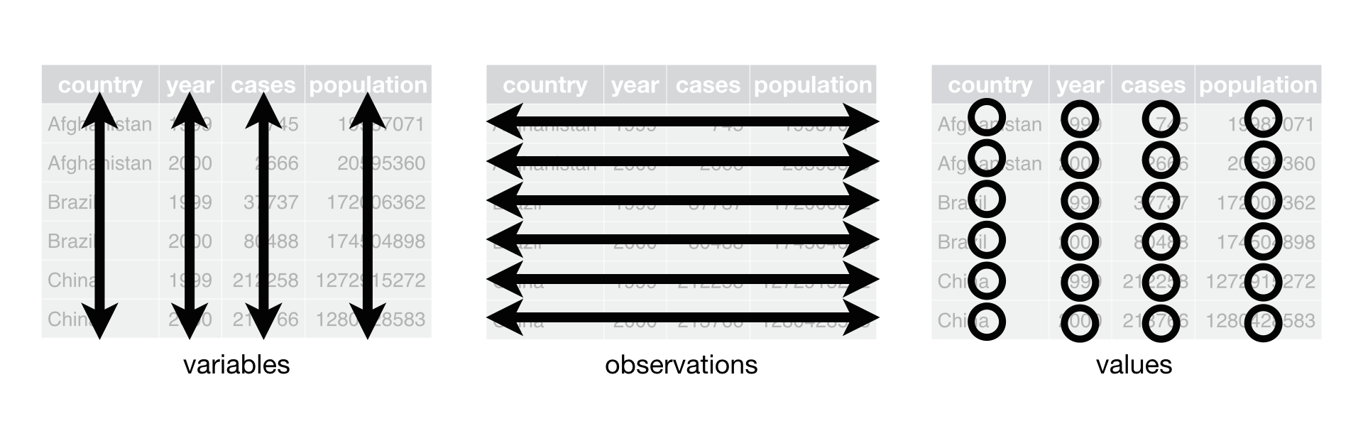
There are three inter-correlated rules which make a dataset tidy:
- Each variable must have its own column.
- Each observation must have its own row.
- Each value must have its own cell.
There are some very real reasons why you would encounter untidy data:
Most people aren’t familiar with the principles of tidy data, and it’s hard to derive them yourself unless you spend a lot of time working with data.
Data is often organised to facilitate some use other than analysis. For example, data is often organised to make entry as easy as possible.
The tidyr package can help you create tidy datasets. A full review of the functions in tidyr is beyond the scope of this workshop. Have a look at the cheatsheet to get started. Just know that the package is available to help create tidy data.
For the example tables above, only the first table is tidy. The second table, although not technically tidy (variables spread across rows), is still a useful format that we’ll work with later. We’ll talk about how to manipulate a dataset to work with both formats using two functions from tidyr: pivot_longer() and pivot_wider().
3.6.1 Values as column names
A common problem is a dataset where some of the column names are not names of variables, but values of a variable. Take table4a: the column names 1999 and 2000 represent values of the year variable, and each row represents two observations, not one.
table4a# A tibble: 3 × 3
country `1999` `2000`
<chr> <dbl> <dbl>
1 Afghanistan 745 2666
2 Brazil 37737 80488
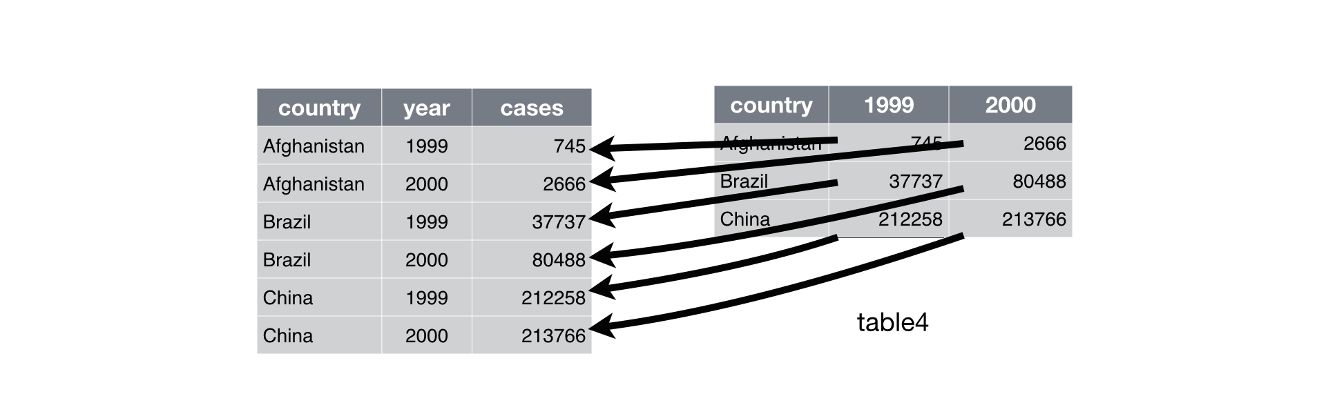
3 China 212258 213766To tidy a dataset like this, we need to combine those columns into a new pair of variables. To describe that operation we need three parameters:
The set of columns that represent values, not variables. In this example, those are the columns
1999and2000.The name of the variable whose values form the column name. Here it is
year.The name of the variable whose values are spread over the cells. Here it’s the number of
cases.
Together those parameters generate the call to pivot_longer():
table4a |>
  pivot_longer(c('1999', '2000'), names_to = "year", values_to = "cases")
# A tibble: 6 × 3
country year cases
<chr> <chr> <dbl>
1 Afghanistan 1999 745
2 Afghanistan 2000 2666
3 Brazil 1999 37737
4 Brazil 2000 80488
5 China 1999 212258
6 China 2000 213766This operation can be graphically demonstrated:
3.6.2 Observations across rows
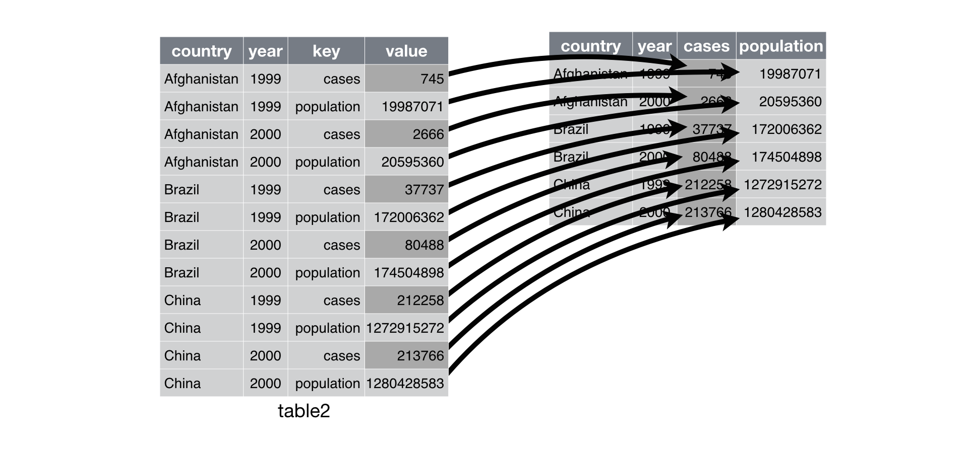
Another problem is when you have a single observation scattered across rows. For example, table2 shows that the number of cases and population is spread across rows where the observation is country and year.
table2# A tibble: 12 × 4
country year type count
<chr> <dbl> <chr> <dbl>
1 Afghanistan 1999 cases 745
2 Afghanistan 1999 population 19987071
3 Afghanistan 2000 cases 2666
4 Afghanistan 2000 population 20595360
5 Brazil 1999 cases 37737
6 Brazil 1999 population 172006362
7 Brazil 2000 cases 80488
8 Brazil 2000 population 174504898
9 China 1999 cases 212258
10 China 1999 population 1272915272
11 China 2000 cases 213766
12 China 2000 population 1280428583To tidy this up, we first analyse the representation in a similar way as before. This time, however, we only need to identify two things:
The column that contains variable names. Here, it’s
type.The column that contains values from multiple variables. Here it’s
count.
Once we’ve figured that out, we can use pivot_wider().
pivot_wider(table2, names_from = 'type', values_from = 'count')# A tibble: 6 × 4
country year cases population
<chr> <dbl> <dbl> <dbl>
1 Afghanistan 1999 745 19987071
2 Afghanistan 2000 2666 20595360
3 Brazil 1999 37737 172006362
4 Brazil 2000 80488 174504898
5 China 1999 212258 1272915272
6 China 2000 213766 1280428583This operation can be graphically demonstrated:
3.7 Exercise 7
Let’s take a look at the fisheries data. Are these data “tidy”? To help with the next few examples, we’ll use pivot_longer() to manipulate the data.
Inspect the fisheries dataset. What are the dimensions (hint:
dim())? What are the names and column types (hint:str())?Use the
pivot_longer()function to move the species columns and count data into two new columns. What value will you use for thenames_toargument? What value will you us for thevalues_toargument? Assign the new dataset to a variable in your environment.Check the dimensions and structure of your new dataset. What’s different?
Click to show/hide solution
# check dimensions, structure
dim(fishdat)
str(fishdat)

# convert fishdat to long format
longdat <- fishdat |>
  pivot_longer(c('Bluefish', 'Common Snook', 'Mullets', 'Pinfish', 'Red Drum', 'Sand Seatrout'), names_to = 'Species', values_to = 'Count')

# check dimensions, structure
dim(longdat)
str(longdat)
3.8 Summarize
The last tool we’re going to learn about in dplyr is the summarize function. As the name implies, this function lets you summarize columns in a dataset. Think of it as a way to condense rows using a summary method of your choice, e.g., what’s the average of the values in a column based on groups in another column?
Let’s use our long form fisheries dataset from exercise 7.
head(longdat)# A tibble: 6 × 8
OBJECTID Reference Sampling_Date yr Gear ExDate Species Count
<dbl> <chr> <date> <dbl> <dbl> <dttm> <chr> <dbl>
1 1550020 TBM19960… 1996-03-20 1996 300 2018-04-12 10:27:38 Bluefi… 0
2 1550020 TBM19960… 1996-03-20 1996 300 2018-04-12 10:27:38 Common… 0
3 1550020 TBM19960… 1996-03-20 1996 300 2018-04-12 10:27:38 Mullets 0
4 1550020 TBM19960… 1996-03-20 1996 300 2018-04-12 10:27:38 Pinfish 0
5 1550020 TBM19960… 1996-03-20 1996 300 2018-04-12 10:27:38 Red Dr… 0
6 1550020 TBM19960… 1996-03-20 1996 300 2018-04-12 10:27:38 Sand S… 1It’s difficult to see patterns in these data until we summarize it some way. Fortunately, the data are setup in a way that let’s us easily summarize by species. We could ask a simple question: how does total catch vary across species (ignoring gear differences, which is a sin in fisheries science)?
We can then use the summarize() function to get the total count. Note the use of the .by argument as a critical piece that defines the groups for summarizing.
by_spp <- summarize(longdat, totals = sum(Count), .by = Species)
by_spp
# A tibble: 6 × 2
Species totals
<chr> <dbl>
1 Bluefish 7
2 Common Snook 3898
3 Mullets 17
4 Pinfish 98182
5 Red Drum 3422
6 Sand Seatrout 7789We can group the dataset by more than one column to get summaries with multiple groups. Here we can look at total count by each unique combination of gear and species.
by_spp_gear <- summarize(longdat, totals = sum(Count), .by = c(Gear, Species))
by_spp_gear
# A tibble: 36 × 3
Gear Species totals
<dbl> <chr> <dbl>
1 300 Bluefish 0
2 300 Common Snook 0
3 300 Mullets 0
4 300 Pinfish 3837
5 300 Red Drum 64
6 300 Sand Seatrout 7072
7 22 Bluefish 0
8 22 Common Snook 0
9 22 Mullets 0
10 22 Pinfish 310
# ℹ 26 more rowsWe can also get more than one summary at a time. The summary function can use any function that operates on a vector. Some common examples include min(), max(), sd(), var(), median(), mean(), and n(). It’s usually good practice to include a summary of how many observations were in each group, so get used to including the n() function.
more_sums <- summarize(longdat,
    n = n(),
    min_count = min(Count),
    max_count = max(Count),
    total = sum(Count),
    .by = Species
  )
more_sums
# A tibble: 6 × 5
Species n min_count max_count total
<chr> <int> <dbl> <dbl> <dbl>
1 Bluefish 2844 0 2 7
2 Common Snook 2844 0 127 3898
3 Mullets 2844 0 5 17
4 Pinfish 2844 0 2530 98182
5 Red Drum 2844 0 123 3422
6 Sand Seatrout 2844 0 560 7789Finally, many of the summary functions we’ve used (e.g., sum(), min(), max(), mean()) will not work correctly if there are missing observations in your data. You’ll see these as NA (or sometimes NaN) entries. You have to use the argument na.rm = T to explicitly tell R how to handle the missing values. Setting na.rm = T says to remove the NA values when summarizing the data.
x <- c(1, 2, NA, 4)
mean(x)
[1] NAmean(x, na.rm = T)[1] 2.333333A quick check for missing values can be done with anyNA. This works on vectors and data frames.
anyNA(x)[1] TRUE3.9 Exercise 8
Now we have access to a several tools in the tidyverse to help us wrangle more effectively. For the final exercise, we’re going to subset our fisheries data and get a summary. Specifically, we’ll filter our data by Gear type 20 and Pinfish, then summarize the average catch across stations.
Using the long data we created in exercise 7, filter the data by Gear type 20 and Pinfish (hint,
filter(Gear == 20 & Species == 'Pinfish').Summarize the count column by taking the average grouped by station (hint,
summarise(ave = mean(Count), .by = Reference)).Which station has the highest average catch of Pinfish (hint,
arrange(ave))?
Click to show/hide solution
sumdat <- longdat |>
  filter(Gear == 20 & Species == 'Pinfish') |>
  summarize(
    ave = mean(Count),
    .by = Reference
  ) |>
  arrange(-ave)
sumdat
3.10 Next time
Now you should be able to answer (or be able to find answers to) the following:
- How are data joined?
- What is tidy data?
- How do I summarize a dataset?
In the next lesson we’ll learn about data visualization and graphics.
3.11 Attribution
Content in this lesson was pillaged extensively from the USGS-R training curriculum here and R for data Science.