R has been around for over thirty years and most of its use has focused on statistical analysis. Tools for spatial analysis have also been developed that allow the use of R as a full-blown GIS with capabilities similar or even superior to commerical software. This lesson will focus on geospatial analysis using the simple features package. We will focus entirely on working with vector data in this lesson, but checkout the terra package if you want to work with raster data in R.
The goals for today are:
Understand the vector data structure
Understand how to import and structure vector data in R
Understand how R stores spatial data using the simple features package
Execute basic geospatial functions in R
5.3 Vector data
Most of us are probably familiar with the basic types of spatial data and their components. We’re going to focus entirely on vector data for this lesson because these data are easily conceptualized as features or discrete objects with spatial information. We’ll discuss some of the details about this later. Raster data, by contrast, are stored in a grid with cells associated with values. Raster data are more common for data with continuous coverage, such as climate or weather layers.
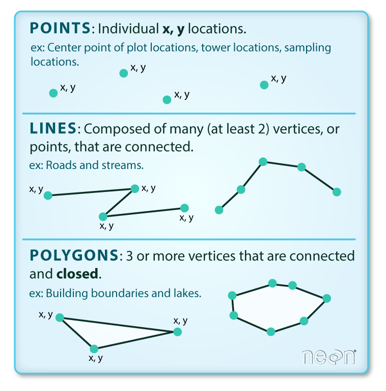
Vector data come in three flavors. The simplest is a point, which is a 0-dimensional feature that can be used to represent a specific location on the earth, such as a single tree or an entire city. Linear, 1-dimensional features can be represented with points (or vertices) that are connected by a path to form a line and when many points are connected these form a polyline. Finally, when a polyline’s path returns to its origin to represent an enclosed 2-dimensional space, such as a forest, watershed boundary, or lake, this forms a polygon.
All vector data are represented similarly, whether they’re points, lines, or polygons. Points are defined by a single coordinate location, whereas a line or polygon include several points with a grouping variable that distinguishes one object from another. In all cases, the aggregate dataset is composed of one or more features of the same type (points, lines, or polygons).
There are two other pieces of information that are included with vector data. The attributes that can be associated with each feature and the coordinate reference system or CRS. The attributes can be any supporting information about a feature, such as a text description or summary data about the features. You can identify attributes as anything in a spatial dataset that is not explicitly used to define the location (or geometry) of the features.
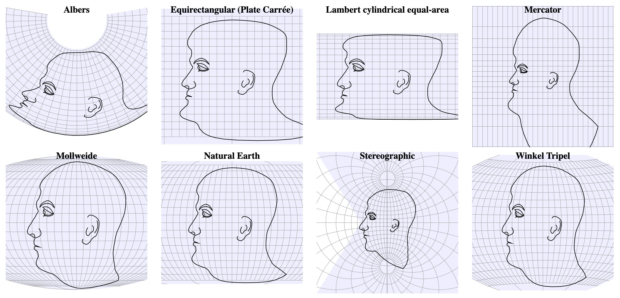
The CRS is used to establish a frame of reference for the locations in your spatial data. The chosen CRS ensures that all features are correctly referenced relative to each other, especially between different datasets. As a simple example, imagine comparing length measurements for two objects where one was measured in centimeters and another in inches. If you didn’t know the unit of measurement, you could not compare relative lengths. The CRS is similar in that it establishes a common frame of reference, but for spatial data. An added complication with spatial data is that location can be represented in both 2-dimensional or 3-dimensional space. This is beyond the scope of this lesson, but for any geospatial analysis you should be sure that:
the CRS is the same when comparing datasets, and
the CRS is appropriate for the region you’re looking at.
spatial data (e.g., latitude, longitude) as points, lines, or polygons
attributes
a coordinate reference system
These are all the pieces of information you need to recognize in your data when working with features in R.
5.4 Simple features
R has a long history of packages for working with spatial data. For many years, the sp package was the standard and most widely used toolset for working with spatial data in R. This package laid the foundation for creating spatial data classes and methods in R, but unfortunately its development predated a lot of the newer tools that are built around the tidyverse. This makes it incredibly difficult to incorporate sp data objects with these newer data analysis workflows.
The simple features or sf package was developed to streamline the use of spatial data in R and to align its functionality with those provided in the tidyverse. The sf package has replaced sp as the fundamental spatial model in R for vector data. A major advantage of sf, as you’ll see, is its intuitive data structure that retains many familiar components of the data.frame (or more accurately, tibble).
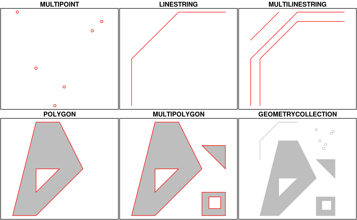
The sf package provides a hierarchical data model that represents a wide range of geometry types - it includes all common vector geometry types and even allows geometry collections, which can have multiple geometry types in a single object. From the first sf package vignette we see:
You’ll notice that these are the same features we described above, with the addition of “multi” features and geometry collections that include more than one type of feature.
5.5 Exercise 12
Let’s get setup for this lesson. We’ll make sure we have the necessary packages installed and loaded. Then we’ll import our datasets.
Open a new script in your RStudio project or within RStudio cloud.
At the top of the script, load the tidyverse, sf, and mapview libraries. Don’t forget you can use install.packages(c('tidyverse', 'sf', 'mapview')) if the packages aren’t installed.
Load the fishdat.csv, statloc.csv, and sgdat.shp datasets from your data folder. For the csv files, use read_csv() and for the shapefile, use the st_read() function from the sf package. The shapefile is seagrass polygon data for Old Tampa Bay in 2016. As before, assign each loaded dataset to an object in your workspace.
Click to show/hide solution
# load librarieslibrary(tidyverse)library(sf)library(mapview)# load the fish datafishdat <-read_csv('data/fishdat.csv')# load the station datastatloc <-read_csv('data/statloc.csv')# load the sgdat shapefilesgdat <-st_read('data/sgdat.shp')
5.6 Creating spatial data with simple features
Now that we’re setup, let’s talk about how the sf package can be used. After the package is loaded, you can check out all of the methods that are available for sf data objects. Many of these names will look familiar if you’re familiar with geospatial analysis methods. We’ll use some of these later.
All of the functions and methods in sf are prefixed with st_, which stands for ‘spatial and temporal’. This is kind of confusing but this is in reference to standard methods available in PostGIS, an open-source backend that is used by many geospatial platforms. An advantage of this prefixing is all commands are easy to find with command-line completion in sf, in addition to having naming continuity with the core, prior software.
There are two ways to create a spatial data object in R, i.e., an sf object, using the sf package.
Directly import a shapefile
Convert an existing R object with latitude/longitude data that represent point features
We’ve already imported a shapefile in Exercise 12, so let’s look at its structure to better understand the sf object. The st_read() function can be used for import. Setting quiet = T will keep R from being chatty when it imports the data.
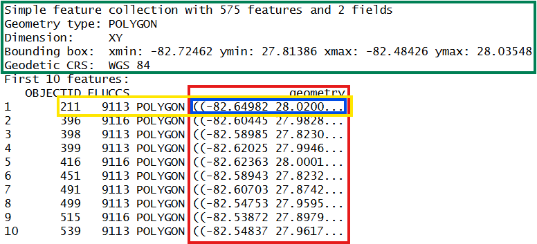
In green, metadata describing components of the sf object
In yellow, a simple feature: a single record, or data.frame row, consisting of attributes and geometry
In blue, a single simple feature geometry (an object of class sfg)
In red, a simple feature list-column (an object of class sfc, which is a column in the data.frame)
We’ve just imported a polygon dataset with 575 features and 2 fields. The dataset uses the WGS 84 geographic CRS (i.e., latitude/longitude). You’ll notice that the actual dataset looks very similar to a regular data.frame, with some interesting additions. The header includes some metadata about the sf object and the geometry column includes the actual spatial information for each feature. Conceptually, you can treat the sf object like you would a data.frame.
Easy enough, but what if we have point data that’s not a shapefile? You can create an sf object from any existing data.frame so long as the data include coordinate information (e.g., columns for longitude and latitude) and you are 100% about the CRS. We can do this with our statloc csv file that we imported.
The st_as_sf() function can be used to make this data.frame into a sf object. We must identify which columns contain the coordinates and provide the CRS information, which is WGS84. You can use the EPSG code 4326 to indicate WGS84.
A big part of working with spatial data is keeping track of coordinate reference systems between different datasets. Remember that meaningful comparisons between datasets are only possible if the CRS is the same.
There are many, many types of reference systems and plenty of resources online that provide detailed explanations of the what and why behind the CRS (see spatialreference.org or this guide from NCEAS). For now, just realize that we can use a simple text string in R to indicate which CRS we want.
5.7 Exercise 13
Our fishdat dataset can be made a simple features spatial object by joining it with the corresponding station data. Let’s join the fishdat and statloc datasets and create an sf object using st_as_sf() function.
Join fishdat to statloc using the left_join() function with by = "Reference" as the key.
Use st_as_sf() to make the joined dataset an sf object. There are two arguments you need to specify with st_as_sf(): coords = c('Longitude', 'Latitude') so R knows which columns in your dataset are the x/y coordinates and crs = 4326 to specifiy the CRS as WGS 84.
When you’re done, inspect the dataset. How many features are there? What type of spatial object is this?
Click to show/hide solution
# Join the dataalldat <-left_join(fishdat, statloc, by ='Reference')# create spatial data objectalldat <-st_as_sf(alldat, coords =c('Longitude', 'Latitude'), crs =4326)# examine the sf objectalldatstr(alldat)
There’s a shortcut for specifying the CRS if you don’t know which one to use. Remember, for spatial analysis make sure to only work with datasets that have the same coordinate reference systems. The st_crs() function tells us the CRS for an existing sf obj.
# check crsst_crs(alldat)
Coordinate Reference System:
User input: EPSG:4326
wkt:
GEOGCRS["WGS 84",
ENSEMBLE["World Geodetic System 1984 ensemble",
MEMBER["World Geodetic System 1984 (Transit)"],
MEMBER["World Geodetic System 1984 (G730)"],
MEMBER["World Geodetic System 1984 (G873)"],
MEMBER["World Geodetic System 1984 (G1150)"],
MEMBER["World Geodetic System 1984 (G1674)"],
MEMBER["World Geodetic System 1984 (G1762)"],
MEMBER["World Geodetic System 1984 (G2139)"],
ELLIPSOID["WGS 84",6378137,298.257223563,
LENGTHUNIT["metre",1]],
ENSEMBLEACCURACY[2.0]],
PRIMEM["Greenwich",0,
ANGLEUNIT["degree",0.0174532925199433]],
CS[ellipsoidal,2],
AXIS["geodetic latitude (Lat)",north,
ORDER[1],
ANGLEUNIT["degree",0.0174532925199433]],
AXIS["geodetic longitude (Lon)",east,
ORDER[2],
ANGLEUNIT["degree",0.0174532925199433]],
USAGE[
SCOPE["Horizontal component of 3D system."],
AREA["World."],
BBOX[-90,-180,90,180]],
ID["EPSG",4326]]
When we created the alldat dataset, we could have used the CRS from the sgdat object that we created in Exercise 12 by using crs = st_crs(sgdat) for the crs argument. This is possible because we have prior knowledge that all of the data use the WGS84 CRS. This is often a quick shortcut for creating an sf object without having to look up the CRS number.
We can verify that both have the same CRS.
# verify the polygon and point data have the same crsst_crs(sgdat)
Coordinate Reference System:
User input: EPSG:4326
wkt:
GEOGCRS["WGS 84",
ENSEMBLE["World Geodetic System 1984 ensemble",
MEMBER["World Geodetic System 1984 (Transit)"],
MEMBER["World Geodetic System 1984 (G730)"],
MEMBER["World Geodetic System 1984 (G873)"],
MEMBER["World Geodetic System 1984 (G1150)"],
MEMBER["World Geodetic System 1984 (G1674)"],
MEMBER["World Geodetic System 1984 (G1762)"],
MEMBER["World Geodetic System 1984 (G2139)"],
ELLIPSOID["WGS 84",6378137,298.257223563,
LENGTHUNIT["metre",1]],
ENSEMBLEACCURACY[2.0]],
PRIMEM["Greenwich",0,
ANGLEUNIT["degree",0.0174532925199433]],
CS[ellipsoidal,2],
AXIS["geodetic latitude (Lat)",north,
ORDER[1],
ANGLEUNIT["degree",0.0174532925199433]],
AXIS["geodetic longitude (Lon)",east,
ORDER[2],
ANGLEUNIT["degree",0.0174532925199433]],
USAGE[
SCOPE["Horizontal component of 3D system."],
AREA["World."],
BBOX[-90,-180,90,180]],
ID["EPSG",4326]]
Finally, you may want to use another coordinate system, such as a projection that is regionally-specific. You can use the st_transform() function to quickly change and/or reproject an sf object. For example, if we want to convert a geographic to UTM projection:
Coordinate Reference System:
User input: +proj=utm +zone=17 +datum=NAD83 +units=m +no_defs
wkt:
PROJCRS["unknown",
BASEGEOGCRS["unknown",
DATUM["North American Datum 1983",
ELLIPSOID["GRS 1980",6378137,298.257222101,
LENGTHUNIT["metre",1]],
ID["EPSG",6269]],
PRIMEM["Greenwich",0,
ANGLEUNIT["degree",0.0174532925199433],
ID["EPSG",8901]]],
CONVERSION["UTM zone 17N",
METHOD["Transverse Mercator",
ID["EPSG",9807]],
PARAMETER["Latitude of natural origin",0,
ANGLEUNIT["degree",0.0174532925199433],
ID["EPSG",8801]],
PARAMETER["Longitude of natural origin",-81,
ANGLEUNIT["degree",0.0174532925199433],
ID["EPSG",8802]],
PARAMETER["Scale factor at natural origin",0.9996,
SCALEUNIT["unity",1],
ID["EPSG",8805]],
PARAMETER["False easting",500000,
LENGTHUNIT["metre",1],
ID["EPSG",8806]],
PARAMETER["False northing",0,
LENGTHUNIT["metre",1],
ID["EPSG",8807]],
ID["EPSG",16017]],
CS[Cartesian,2],
AXIS["(E)",east,
ORDER[1],
LENGTHUNIT["metre",1,
ID["EPSG",9001]]],
AXIS["(N)",north,
ORDER[2],
LENGTHUNIT["metre",1,
ID["EPSG",9001]]]]
Above, we’ve used the “Proj4string” format of the CRS, instead of the EPSG code. This is another perfectly acceptable way to specify a CRS. Also note that transformations can only be done after the original data are correctly imported using the native CRS of the dataset.
5.8 Basic geospatial analysis
Let’s perform some simple geospatial analysis comparing the fisheries data with the seagrass data. As with any analysis, let’s take a look at the data to see what we’re dealing with before we start comparing the two.
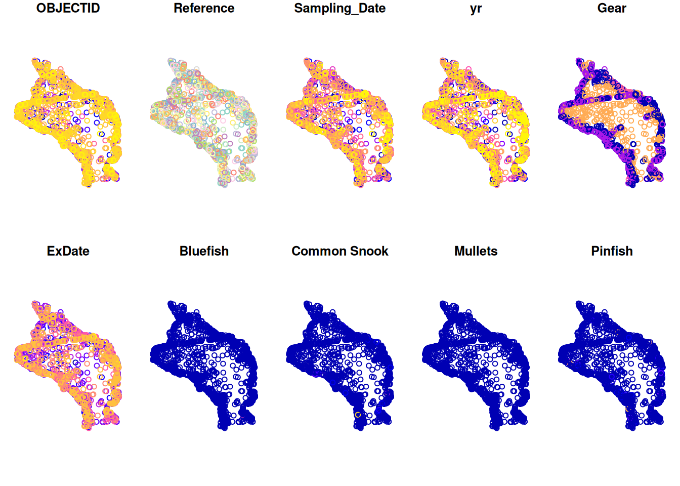
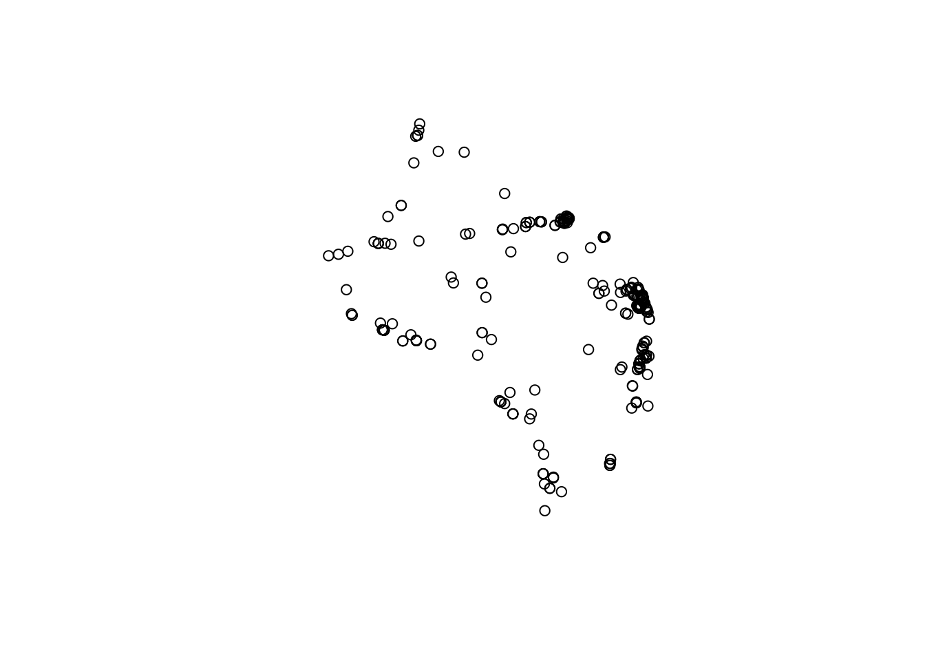
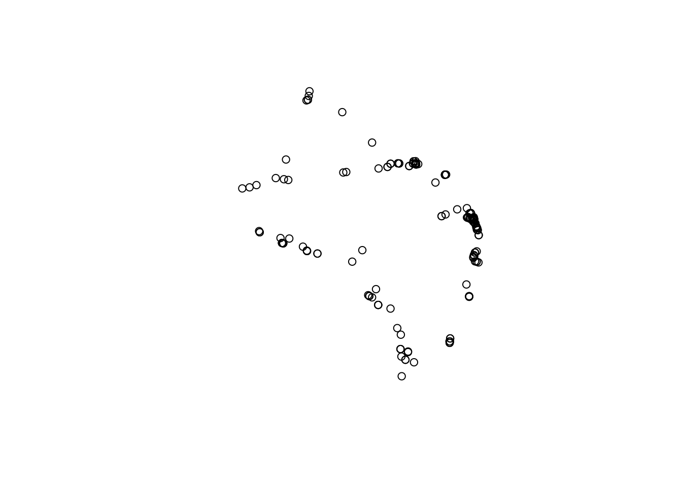
plot(alldat)
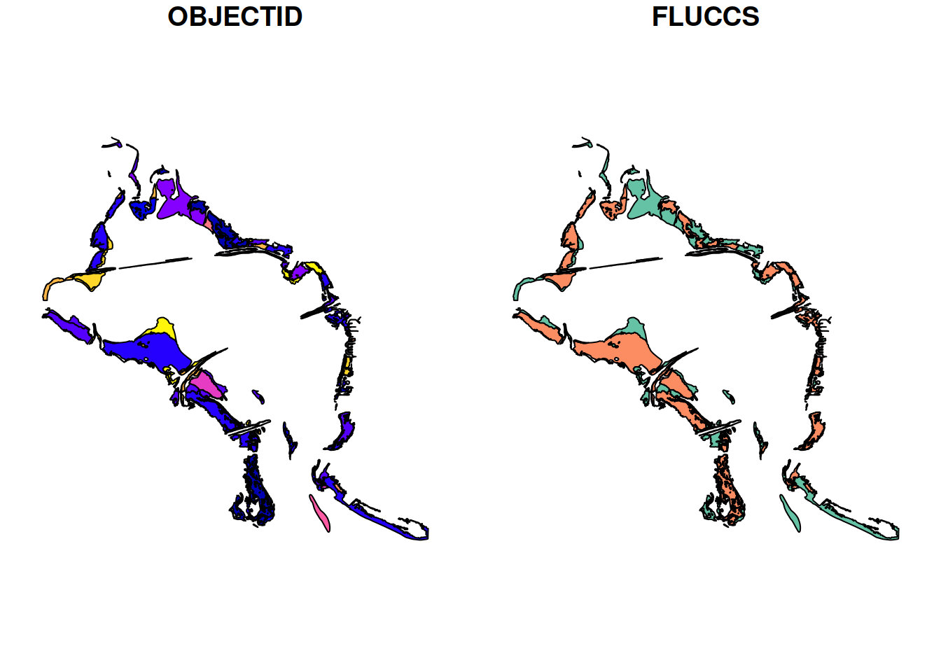
plot(sgdat)
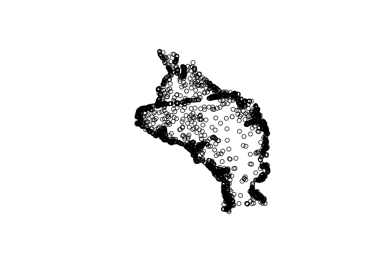
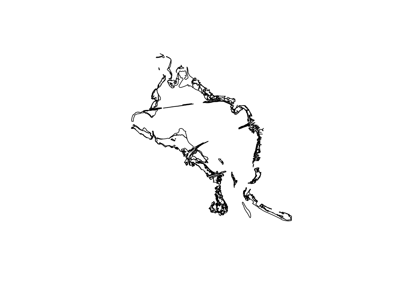
We have lots of stations where fish have been caught and lots of polygons where seagrass has been documented. You’ll also notice that the default plotting method for sf objects is to create one plot per attribute feature. This is intended behavior but sometimes is not that useful (it can also break R if you have many attributes). Maybe we just want to see where the data are located independent of any of the attributes. We can accomplish this by plotting only the geometry of the sf object.
plot(alldat$geometry)
plot(sgdat$geometry)
To emphasize the point that the sf package plays nice with the tidyverse, let’s do a simple filter on the fisheries data to look at only the 2016 data. This is the same year as the seagrass data.
Now let’s use the fisheries data and seagrass polygons to do a quick geospatial analysis. Our simple question is:
How many fish were caught where seagrass was observed in 2016?
The first task is to subset the 2016 fisheries data by locations where seagrass was observed. There are a few ways we can do this. The first is to make a simple subset where we filter the station locations using a spatial overlay with the seagrass polygons. With this approach we can see which stations were located over seagrass, but we don’t know which polygons they’re located in for the seagrass data (i.e., this is not a true spatial intersection).
The second and more complete approach is to intersect the two data objects to subset and combine the attributes. We can use st_intersection() to both overlay and combine the attribute fields from the two data objects.
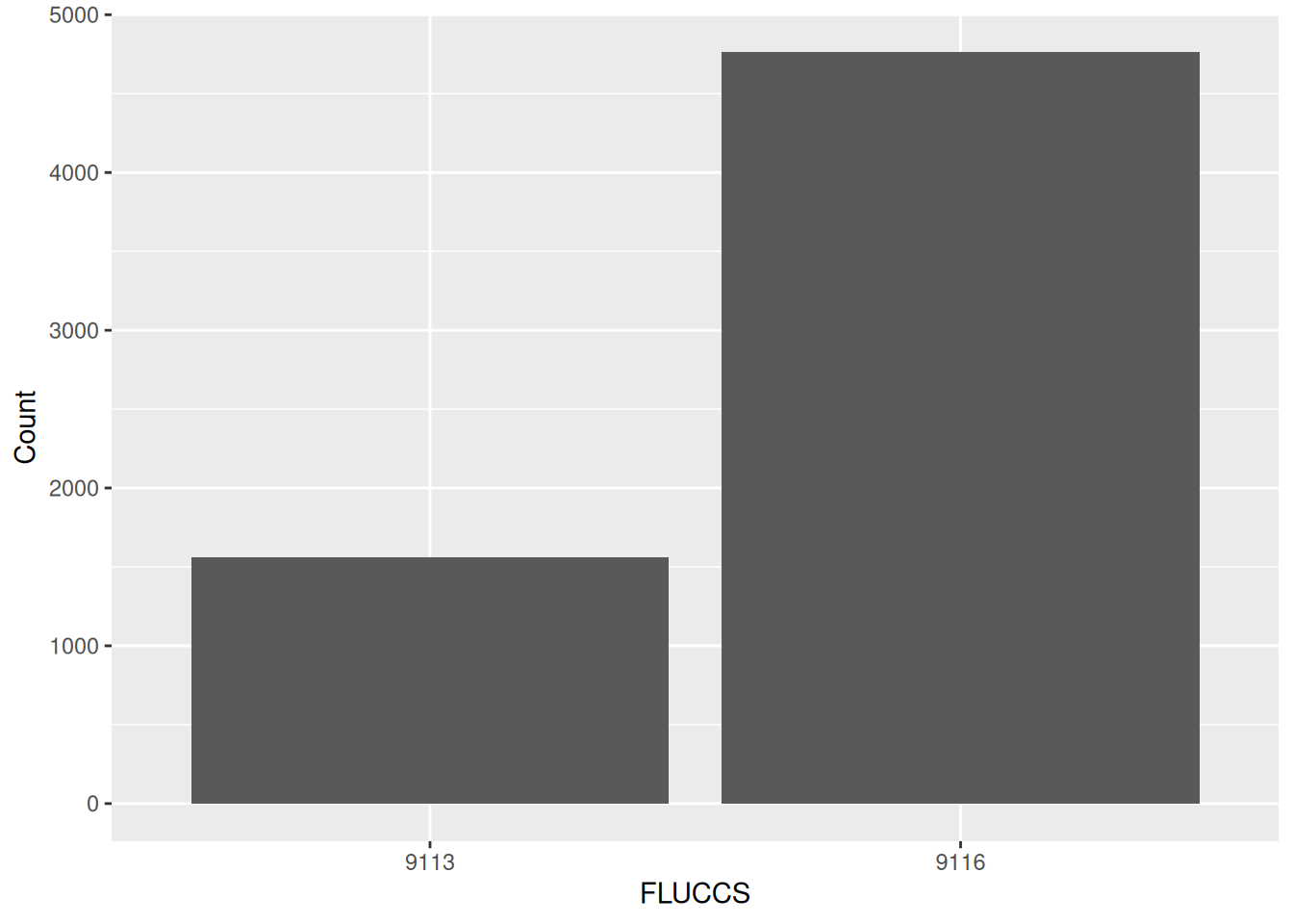
Now we can easily see which stations are in which seagrass polygon. We can use some familiar tools from dplyr to get the aggregate catch data for the different polygon counts. Specifically, the FLUCCS attribute identifies seagrass polygons as continuous (9116) or patchy (9113) (metadata here). Maybe we want to summarise species counts by seagrass polygon type. Here, we need to specify the FLUCCS grouping variable outside of the summarize function.
Notice that we’ve retained the sf data structure in the aggregated dataset but the structure is now slightly different, both in the attributes and the geometry column. We now have only two attributes, FLUCCS and Count. The geometry column is retained but now is aggregated to a multipoint object where all points in continous or patchy seagrass are grouped by row. This is a really powerful feature of sf: spatial attributes are retained during the wrangling process.
We can also visualize this information with ggplot2. This plot shows how many pinfish were caught in the two seagrass coverage categories for all of Old Tampa Bay (9113: patchy, 9116: continuous).
ggplot(fish_cnt, aes(x = FLUCCS, y = Count)) +geom_bar(stat ='identity')
This is not a groundbreaking plot, but we can clearly see that pinfish are more often found in dense seagrass beds (9116).
5.9 Quick mapping
Cartography or map-making is also very doable in R. Like most applications, it takes very little time to create something simple, but much more time to create a finished product. We’ll focus on the simple process using ggplot2 and the mapview package just to get you started. Both packages work “out-of-the-box” with sf data objects.
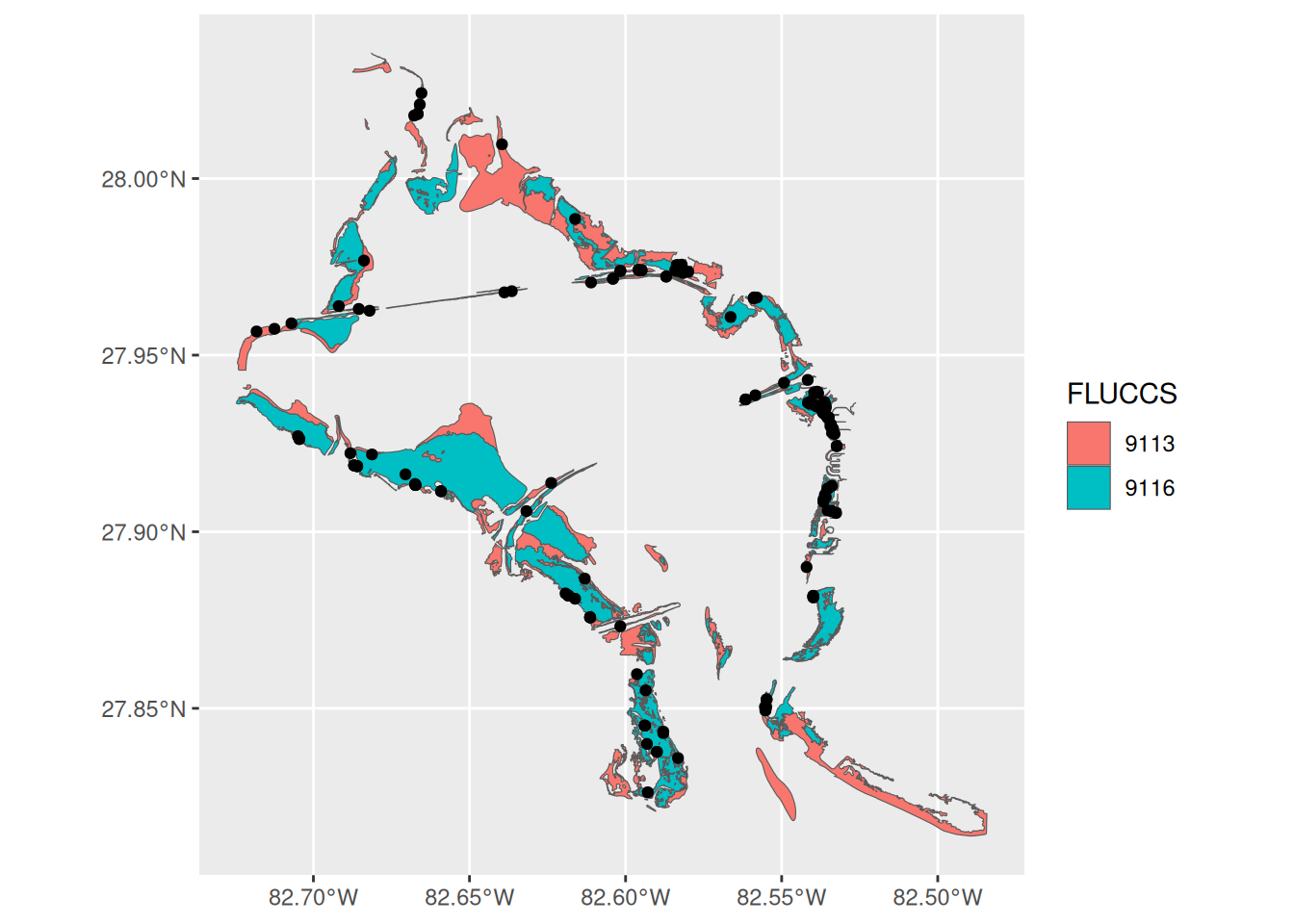
For ggplot2, all we need is to use the geom_sf() geom.
# use ggplot with sf objectsggplot() +geom_sf(data = sgdat, aes(fill = FLUCCS)) +geom_sf(data = fish_int)
The mapview packages lets us create interactive maps to zoom and select data. Note that we can also combine separate mapview objects with the + operator.
mapview(sgdat, zcol ='FLUCCS') +mapview(fish_int)
There’s a lot more we can do with mapview but the point is that these maps are incredibly easy to make with sf objects and they offer a lot more functionality than static plots.
5.10 Exercise 14
We’ll spend the remaining time getting more comfortable with basic geospatial analysis and mapping in R.
Start by filtering the alldat object you created in Exercise 13 to retain only 2016 data. Intersect the filtered data with the sgdat object using st_intersection().
Create a map of this intersected object using mapview(). Use the zcol argument to map the color values to different attributes in your dataset, e.g., Pinfish or Bluefish.
Try combining the map you made in the last step with one for seagrass (hint: mapview() + mapview()).
Understand how to import and structure vector data in R
Understand how R stores spatial data using the simple features package
Execute basic geospatial functions in R
This concludes our training workshop. I hope you’ve enjoyed the material and found the content useful. Please continue to use this website as a resource for developing your R skills and checkout our Data and Resources page for additional learning material.