Appendix B — Introduction to R

B.1 RStudio

RStudio is the go-to Interactive Development Environment (IDE) for R. Rstudio includes many features to improve the user’s experience.

Let’s get familiar with RStudio.

B.1.1 Open R and RStudio

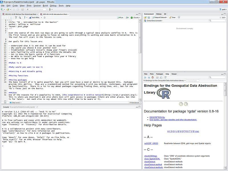
Find the RStudio shortcut on your computer and fire it up. You should see something like this:

There are four panes in RStudio:

• Source: Your primary window for writing code to send to the console, this is where you write and save R “scripts”
• Console: This is where code is executed in R
• Environment, History, etc.: A tabbed window showing your working environment, code execution history, and other useful things
• Files, plots, etc.: A tabbed window showing a file explorer, a plot window, list of installed packages, help files, and viewer

B.1.2 Scripting

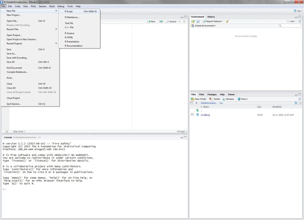
In most cases, you will not enter and execute code directly in the console. Code can be written in a script and then sent directly to the console.

Open a new script from the File menu…

B.1.3 Executing code in RStudio

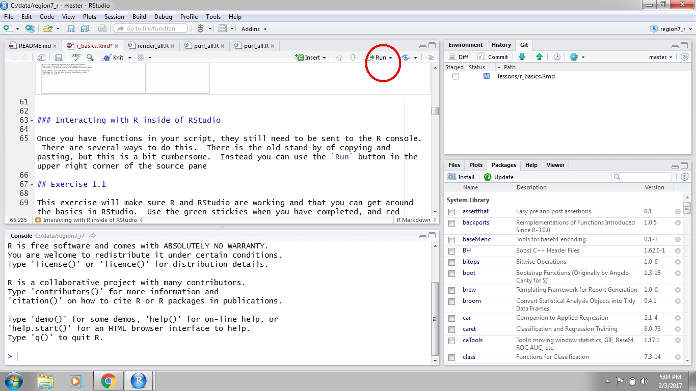
After you write code in an R script, it can be sent to the Console to run the code. There are two ways to do this. First, you can hit the Run button at the top right of the scripting window. Second, you can use ctrl+enter (cmd+enter on a Mac). Either option will run the line(s) of script that are selected.

B.2 R language fundamentals

R is built around functions. The basic syntax of a function follows the form: function_name(arg1, arg2, ...).

With the base install, you will gain access to many functions (2356, to be exact). Some examples:

# print
print("hello world!")

[1] "hello world!"

# sequence
seq(1, 10)

 [1]  1  2  3  4  5  6  7  8  9 10

# random numbers
rnorm(100, mean = 10, sd = 2)

  [1]  8.215288 15.752656  9.363572  7.096341 13.345945 11.925304  7.507875
  [8] 10.174912  9.174257  8.487599 12.682729 12.232503 12.734577  9.118885
 [15]  8.426590 10.071299 10.622701  8.664416  8.383698  6.203215 10.317726
 [22] 10.093311 10.460603 10.106924 14.083985  9.923904 10.377201 11.011934
 [29] 12.984380  9.246387  8.747104  9.296439 10.366758 10.874941 10.715875
 [36]  8.987754  8.966694  7.613422 12.703589 11.226438  8.302283 13.723784
 [43] 13.040958  7.067523  8.381173  9.294102  7.023449  7.952067 12.535866
 [50] 10.795284 10.832161  8.966341 10.484411 11.099160 12.223793  8.223438
 [57]  7.062739 11.312607 10.525698 10.062231  9.999916 10.776142 10.400968
 [64]  9.842209 10.751344  9.978962  9.005056  6.222508  8.069472  8.449853
 [71] 11.131733 15.013956  8.401588 10.487518 11.220381 11.580249 10.607620
 [78] 11.078196  8.687162 10.964094  8.299364  8.952931 11.825084  9.399767
 [85] 10.931394  8.317562 13.873030 11.286575 11.061332 10.777481 12.271623
 [92] 11.604692  8.403873  7.693848 10.510489 10.815880 12.686081 11.144177
 [99]  9.061215  8.391056

# average 
mean(rnorm(100))

[1] 0.04233977

# sum
sum(rnorm(100))

[1] 0.38761

Very often you will see functions used like this:

my_random_sum <- sum(rnorm(100))

The first part of the line is the name of an object that you make up. The second bit, <-, is the assignment operator. This tells R to take the result of sum(rnorm(100)) and store it in an object named, my_random_sum. It is stored in the environment and can be used by just executing it’s name in the console.

my_random_sum

[1] -11.83266

B.2.1 What is the environment?

There are two outcomes when you run code. First, the code will simply print output directly in the console. Second, there is no output because you have stored it as a variable using <-. Output that is stored is saved in the environment. The environment is the collection of named objects that are stored in memory for your current R session.

B.3 Packages

The base installation of R is quite powerful. Packages allow you to include new methods for use in R.

B.3.1 CRAN

Many packages are available on CRAN, The Comprehensive R Archive Network. This is where you download R and also where most will gain access to packages. As of 2025-03-14, there are 22188 packages on CRAN!

B.3.2 Installing packages

When a package gets installed, that means the source code is downloaded and put into your library. A default library location is set for you.

We use the install.packages() function to download and install a package. Here, we install the readxl package, used below, which is used to upload data from and Excel file.

install.packages("readxl")

You should see some text in the R console showing progress of the installation and a prompt after installation is done.

After installation, you can load a package using the library() function. This makes all functions in a package available for you to use.

library(readxl)

An important aspect of packages is that you only need to download them once, but every time you start RStudio you need to load them with the library() function.

B.4 Data structures in R

Now we can talk about R data structures. Simply put, a data structure is a way for programming languages to handle information storage.

B.4.1 Vectors (one-dimensional data)

The basic data format in R is a vector - a one-dimensional grouping of elements that have the same type. These are all vectors and they are created with the c (concatenate) function:

dbl_var <- c(1, 2.5, 4.5)
int_var <- c(1L, 6L, 10L)
log_var <- c(TRUE, FALSE, T, F)
chr_var <- c("a", "b", "c")

The four types of vectors are double (or numeric), integer, logical, and character. The following functions can return useful information about the vectors:

class(dbl_var)

[1] "numeric"

length(log_var)

[1] 4

B.4.2 Data frames (two-dimensional data)

A collection of vectors represented as one data object are often described as two-dimensional data, like a spreadsheet, or in R speak, a data frame. Here’s a simple example:

ltrs <- c("a", "b", "c")
nums <- c(1, 2, 3)
logs <- c(T, F, T)
mydf <- data.frame(ltrs, nums, logs)
mydf

  ltrs nums  logs
1    a    1  TRUE
2    b    2 FALSE
3    c    3  TRUE

The only constraints required to make a data frame are:

1. Each column (vector) contains the same type of data

2. The number of observations in each column is equal.

B.5 Getting your data into R

It is the rare case when you manually enter your data in R. Most data analysis workflows typically begin with importing a dataset from an external source. We’ll be using read_excel() function from the readxl package.

We can import the ExampleSites.xlsx dataset as follows. Note the use of a relative file path. You can see what R is using as your “working directory” using the getwd() function.

sitdat <- read_excel("data/ExampleSites.xlsx")

Let’s explore the dataset a bit.

# get the dimensions
dim(sitdat)

[1] 11  5

# get the column names
names(sitdat)

[1] "Monitoring Location ID"        "Monitoring Location Name"     
[3] "Monitoring Location Latitude"  "Monitoring Location Longitude"
[5] "Location Group"               

# see the first six rows
head(sitdat)

# A tibble: 6 × 5
  `Monitoring Location ID` `Monitoring Location Name` Monitoring Location Lati…¹
  <chr>                    <chr>                                           <dbl>
1 ABT-026                  Rte 2, Concord                                   42.5
2 ABT-062                  Rte 62, Acton                                    42.4
3 ABT-077                  Rte 27/USGS, Maynard                             42.4
4 ABT-144                  Rte 62, Stow                                     42.4
5 ABT-237                  Robin Hill Rd, Marlboro                          42.3
6 ABT-301                  Rte 9, Westboro                                  42.3
# ℹ abbreviated name: ¹​`Monitoring Location Latitude`
# ℹ 2 more variables: `Monitoring Location Longitude` <dbl>,
#   `Location Group` <chr>

# get the overall structure
str(sitdat)

tibble [11 × 5] (S3: tbl_df/tbl/data.frame)
 $ Monitoring Location ID       : chr [1:11] "ABT-026" "ABT-062" "ABT-077" "ABT-144" ...
 $ Monitoring Location Name     : chr [1:11] "Rte 2, Concord" "Rte 62, Acton" "Rte 27/USGS, Maynard" "Rte 62, Stow" ...
 $ Monitoring Location Latitude : num [1:11] 42.5 42.4 42.4 42.4 42.3 ...
 $ Monitoring Location Longitude: num [1:11] -71.4 -71.4 -71.4 -71.5 -71.6 ...
 $ Location Group               : chr [1:11] "Assabet" "Assabet" "Assabet" "Assabet" ...

You can also view a dataset in a spreadsheet style using the View() function:

View(sitdat)

B.6 Summary

In this intro we learned about R and Rstudio, some of the basic syntax and data structures in R, and how to import files. You’ll be able to follow the rest of the workshop with this knowledge.