Plot mean AMBI scores over time by bay segment

Usage

show_ambitrend(
  ambiscr,
  ambiscr_tb = NULL,
  bay_segment = c("HB", "OTB", "MTB", "LTB", "TCB", "MR", "BCB", "All"),
  yrrng = c(1993, 2024),
  yscl = TRUE,
  plotly = FALSE,
  width = NULL,
  height = NULL
)

Arguments

ambiscr: input data frame as returned by anlz_ambiscr, the AMBI variant (conventional or Tampa Bay-specific) is detected automatically from the column names
ambiscr_tb: optional second input data frame from anlz_ambiscr for overlaying the other AMBI variant on the same plot
bay_segment: chr string for the bay segment, one to many of "HB", "OTB", "MTB", "LTB", "TCB", "MR", "BCB", "All". When multiple segments are selected (or "All"), scores are averaged across all sites in the selected segments.
yrrng: numeric vector of length two indicating the year range to plot
yscl: logical indicating whether the y-axis should span the full adjusted AMBI range (0 to 10, default TRUE) or be scaled to the range of the annual means (FALSE)
plotly: logical if the plot is created using plotly
width: numeric for width of the plot in pixels, only applies if plotly = TRUE
height: numeric for height of the plot in pixels, only applies if plotly = TRUE

Value

A ggplot object showing mean adjusted AMBI scores by year if plotly = FALSE, otherwise a plotly object

Details

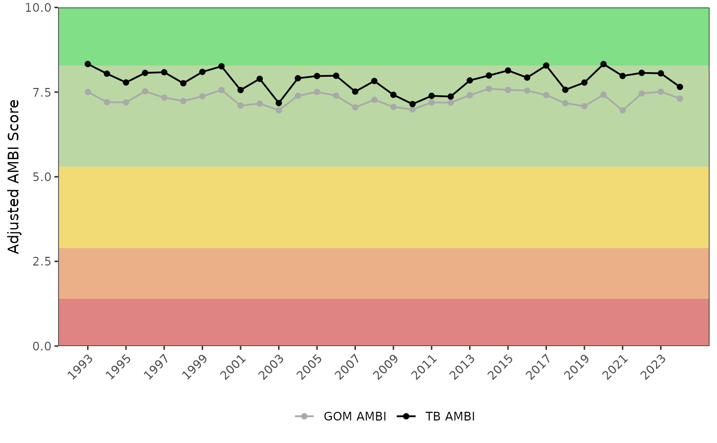
The background of the plot is shaded by AMBI pollution category using the adjusted score thresholds (0-10 scale, higher = healthier): Unpolluted (8.29-10, dark green), Slightly Polluted (5.29-8.29, light green), Meanly Polluted (2.89-5.29, yellow), Heavily Polluted (1.39-2.89, orange), and Extremely Polluted (0-1.39, red).

Only sampling funded by TBEP and as part of the routine EPC benthic monitoring program are included.

If both ambiscr and ambiscr_tb are provided, both series are shown on the same plot with dark grey used for the first series and black for the second. The AMBI variant for each input is detected automatically from the column names (AMBI or TBAMBI).

Examples

ambiscr    <- anlz_ambiscr(benthicdata)
ambiscr_tb <- anlz_ambiscr(benthicdata, type = 'AMBI-TB')
show_ambitrend(ambiscr, ambiscr_tb)