Background
The Tampa Bay Nekton Index (TBNI) [1,2]) is a multimetric assessment method that quantifies the ecological health of the nekton community in Tampa Bay. The index provides a complementary approach to evaluating environmental condition that is supported by other assessment methods currently available for Tampa Bay (e.g., water quality report card, Benthic index, etc.). The tbeptools package includes several functions described below to import data required for the index, analyze the data to calculate metrics and index scores, and plot the results to view trends over time. Each of the functions are described in detail below.
The TBNI uses catch data from the Florida Fish and Wildlife Conservation Commission (FWC) Fish and Wildlife Research Institute’s (FWRI) Fisheries-Independent Monitoring (FIM) program. Catch results from a center-bag seine have the longest and most consistent record in the FIM database and were used to develop the TBNI. These include counts and taxa identification for individuals caught in near shore areas, generally as early recruits, juveniles, and smaller-bodied nekton. All fish and selected invertebrates are identified to the lowest possible taxon (usually species), counted, and a subset are measured. Current protocols were established in 1998 and TBNI estimates are unavailable prior to this date.
Data import and included datasets
Data required for calculating TBNI scores can be imported into the
current R session using the read_importfim() function. This
function downloads the latest FIM file from an FTP site if the data have
not already been downloaded to the location specified by the input
arguments.
To download the data, first create a character path for the location
of the file. If one does not exist, specify a desired location and name
for the downloaded file. Here, we want to put the file on the desktop in
our home directory and name it fimdata.csv.
csv <- '~/Desktop/fimdata.csv'
fimdata <- read_importfim(csv)
Running the above code will return the following error:
#> Error in read_importfim(csv) : file.exists(csv) is not TRUEWe get an error message from the function indicating that the file is
not found. This makes sense because the file doesn’t exist yet, so we
need to tell the function to download the latest file. This is done by
changing the download_latest argument to TRUE
(the default is FALSE).
fimdata <- read_importfim(csv, download_latest = T)
#> File ~/Desktop/fimdata.csv does not exist, replacing with downloaded file...Now we get an indication that the file on the server is being
downloaded. When the download is complete, we’ll have the data
downloaded and saved to the fimdata object in the current R
session.
If we try to run the function again after downloading the data from the server, we get the following message. This check is done to make sure that the data are not unnecessarily downloaded if the current matches the file on the server.
fimdata <- read_importfim(csv, download_latest = T)
#> File is current..Every time that tbeptools is used to work with the FIM data,
read_importfim() should be used to import the data. You
will always receive the message File is current... if your
local file matches the one on the server. However, new data are
regularly collected and posted on the server. If
download_latest = TRUE and your local file is out of date,
you will receive the following message:
#> Replacing local file with current...After the data are successfully imported, you can view them from the assigned object:
head(fimdata)
#> # A tibble: 6 × 19
#>   Reference    Sampling_Date Latitude Longitude Zone   Grid NODCCODE  Year Month
#>   <chr>        <date>           <dbl>     <dbl> <chr> <int> <chr>    <dbl> <dbl>
#> 1 TBM19980109… 1998-01-09        28.0     -82.7 A        31 8747020…  1998     1
#> 2 TBM19980109… 1998-01-09        28.0     -82.7 A        31 8805030…  1998     1
#> 3 TBM19980109… 1998-01-09        27.9     -82.7 A        62 6177010…  1998     1
#> 4 TBM19980109… 1998-01-09        27.9     -82.7 A        63 9998000…  1998     1
#> 5 TBM19980109… 1998-01-09        27.9     -82.6 A        65 8820020…  1998     1
#> 6 TBM19980109… 1998-01-09        27.9     -82.6 A        65 8826020…  1998     1
#> # ℹ 10 more variables: Total_N <dbl>, ScientificName <chr>,
#> #   Include_TB_Index <chr>, Hab_Cat <chr>, Est_Cat <chr>, Est_Use <chr>,
#> #   Feeding_Cat <chr>, Feeding_Guild <chr>, Selected_Taxa <chr>,
#> #   bay_segment <chr>
The imported data are formatted for calculating the TBNI. The columns
include a Reference for the FIM sampling site, the sampling
date, sampling Zone, sampling Grid,
NODCCODE as a unique identifier for species, sample year,
sample month, total catch as Total_N, scientific name, a
column indicating if the species is included in the index, and several
columns indicating species-specific information required for the
metrics. For the final columns, a separate lookup table is provided in
the package that is merged with the imported FIM data. This file,
tbnispp, can be viewed anytime the package is loaded:
head(tbnispp)
#>      TSN   NODCCODE               ScientificName Include_TB_Index Hab_Cat
#> 1 173245 8860030201 Acanthostracion quadricornis                Y       B
#> 2 172986 8858030202             Achirus lineatus                Y       B
#> 3 160978 8713070101           Aetobatus narinari                Y       B
#> 4 161121 8739010101                Albula vulpes                Y       P
#> 5  96600 6179140000               Alpheidae spp.                N       B
#> 6 173131 8860020101           Aluterus schoepfii                Y       B
#>   Est_Cat Est_Use Feeding_Cat Feeding_Guild Selected_Taxa
#> 1      MS       O          TS            ZB             N
#> 2      ES       O          TS            ZB             N
#> 3      MS       F          TS            ZB             N
#> 4      MS       S          TS            ZB             Y
#> 5                          DV            DV             N
#> 6      MS       F          TS            HV             N
The read_importfim() function can also return a simple
features object of sampled stations in the raw FIM data by setting .
These data are matched to the appropriate bay segments for tabulating
TBNI scores. The resulting dataset indicates where sampling has occurred
and can be mapped with the mapview() function. For ease of
use, a dataset named fimstations is included in
tbeptools.
fimstations <- read_importfim(csv, download_latest = TRUE, locs = TRUE)
mapview(fimstations, zcol = 'bay_segment')
The read_importfim() function processes the observed
data as needed for the TBNI, including merging the rows with the
tbnispp and fimstations data. Once imported,
the metrics and scores can be calculated.
Calculating metrics and TBNI scores
Metrics and scores for the Tampa Bay Nekton Index can be calculated
using two functions. The anlz_tbnimet() function calculates
all raw metrics and the anlz_tbniscr() function calculates
scored metrics and the final TBNI score. Both functions use the imported
and formatted FIM data as input.
The TBNI includes five metrics that were sensitive to stressor gradients and provide unique information about Nekton community response to environmental conditions. The metrics include:
NumTaxa: Species richnessBenthicTaxa: Species richness for benthic taxaTaxaSelect: Number of “selected” species (i.e., commercially and/or recreationally important)NumGuilds: Number of trophic guildsShannon: Shannon Diversity (H)
Raw metrics are first calculated from the observed data and then scaled to a standard score from 0 - 10 by accounting for expected relationships to environmental gradients and 5th/95th percentiles of the distributions. The final TBNI score is the summed average of the scores ranging from 0 - 100.
The raw metrics, scored metrics, and final TBNI score is returned
with the anlz_tbniscr() function.
tbniscr <- anlz_tbniscr(fimdata)
head(tbniscr)
#> # A tibble: 6 × 16
#>   Reference      Year Month Season bay_segment TBNI_Score NumTaxa ScoreNumTaxa
#>   <chr>         <dbl> <dbl> <chr>  <chr>            <dbl>   <dbl>        <dbl>
#> 1 TBM1998010906  1998     1 Winter OTB                 18       2            2
#> 2 TBM1998010910  1998     1 Winter OTB                 14       1            1
#> 3 TBM1998010912  1998     1 Winter OTB                  0       0            0
#> 4 TBM1998010914  1998     1 Winter OTB                 20       2            2
#> 5 TBM1998010915  1998     1 Winter MTB                 46       4            4
#> 6 TBM1998010917  1998     1 Winter MTB                 24       2            2
#> # ℹ 8 more variables: BenthicTaxa <dbl>, ScoreBenthicTaxa <dbl>,
#> #   TaxaSelect <dbl>, ScoreTaxaSelect <dbl>, NumGuilds <dbl>,
#> #   ScoreNumGuilds <dbl>, Shannon <dbl>, ScoreShannon <dbl>
The five metrics chosen for the TBNI were appropriate for the Tampa
Bay dataset and were selected from a larger pool of candidate metrics.
All potential metrics can be calculated using the
anlz_tbnimet() function. These metrics can be used in
standalone assessments or for developing a Nekton index outside of Tampa
Bay. The argument all = TRUE must be used to return all
metrics, otherwise only the selected five for the TBNI are returned.
tbnimet <- anlz_tbnimet(fimdata, all = T)
head(tbnimet)
#> # A tibble: 6 × 37
#>   Reference      Year Month Season bay_segment NumTaxa NumIndiv Shannon Simpson
#>   <chr>         <dbl> <dbl> <chr>  <chr>         <dbl>    <dbl>   <dbl>   <dbl>
#> 1 TBM1998010906  1998     1 Winter OTB               2       17   0.362    1.26
#> 2 TBM1998010910  1998     1 Winter OTB               1        1   0        1
#> 3 TBM1998010912  1998     1 Winter OTB               0        0   0        0
#> 4 TBM1998010914  1998     1 Winter OTB               2        2   0.693    2
#> 5 TBM1998010915  1998     1 Winter MTB               4       11   1.16     2.81
#> 6 TBM1998010917  1998     1 Winter MTB               2        5   0.500    1.47
#> # ℹ 28 more variables: Pielou <dbl>, TaxaSelect <dbl>, NumGuilds <dbl>,
#> #   TSTaxa <dbl>, TGTaxa <dbl>, BenthicTaxa <dbl>, PelagicTaxa <dbl>,
#> #   OblTaxa <dbl>, MSTaxa <dbl>, ESTaxa <dbl>, SelectIndiv <dbl>, Taxa90 <dbl>,
#> #   TSAbund <dbl>, TGAbund <dbl>, BenthicAbund <dbl>, PelagicAbund <dbl>,
#> #   OblAbund <dbl>, ESAbund <dbl>, MSAbund <dbl>, Num_LR <dbl>, PropTG <dbl>,
#> #   PropTS <dbl>, PropBenthic <dbl>, PropPelagic <dbl>, PropObl <dbl>,
#> #   PropMS <dbl>, PropES <dbl>, PropSelect <dbl>
Plotting results
The TBNI scores can be viewed as annual averages using the
show_tbniscr(), show_tbniscrall() and
show_tbnimatrix() functions. The
show_tbniscr() creates a line graph of values over time for
each bay segment, whereas the show_tbniscrall() function
plots an overall average across bay segments over time. The
show_tbnimatrix() plots the annual bay segment averages as
categorical values in a conventional “stoplight” graphic. The input to
each function is the output from the anlz_tbniscr()
function.
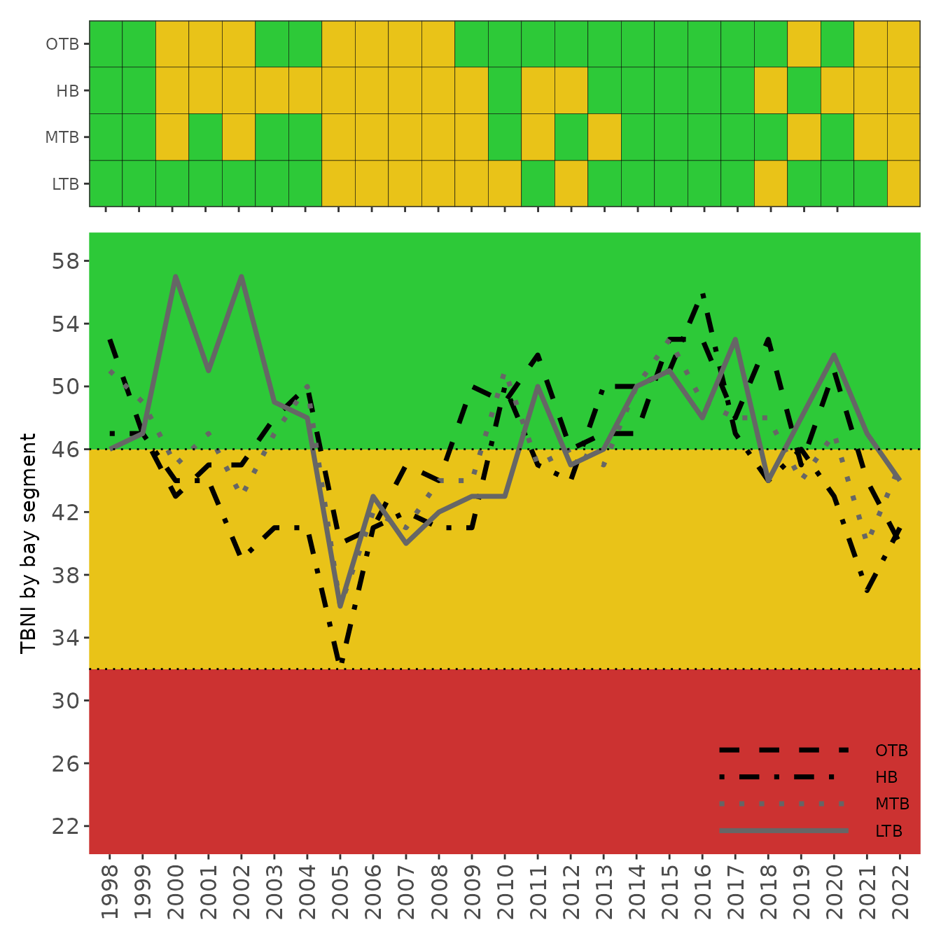
show_tbniscr(tbniscr)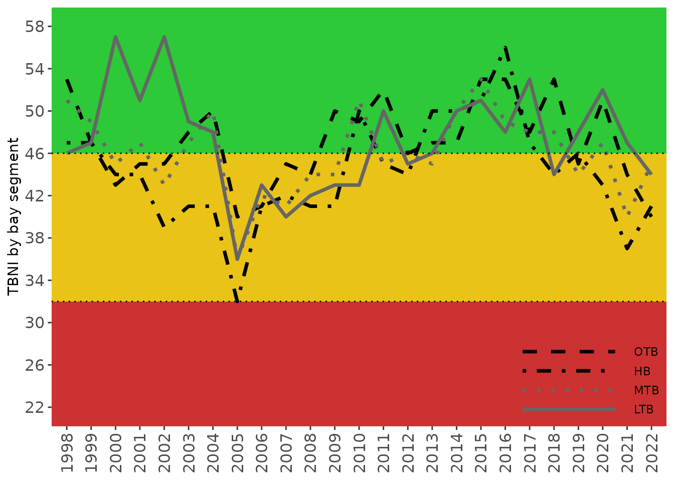
show_tbniscrall(tbniscr)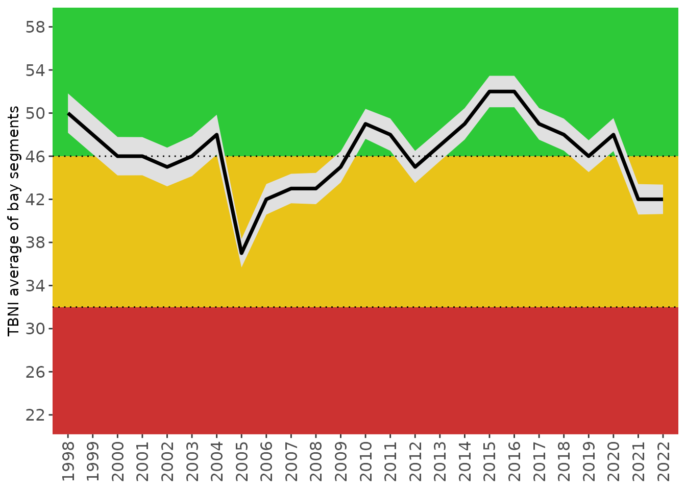
show_tbnimatrix(tbniscr)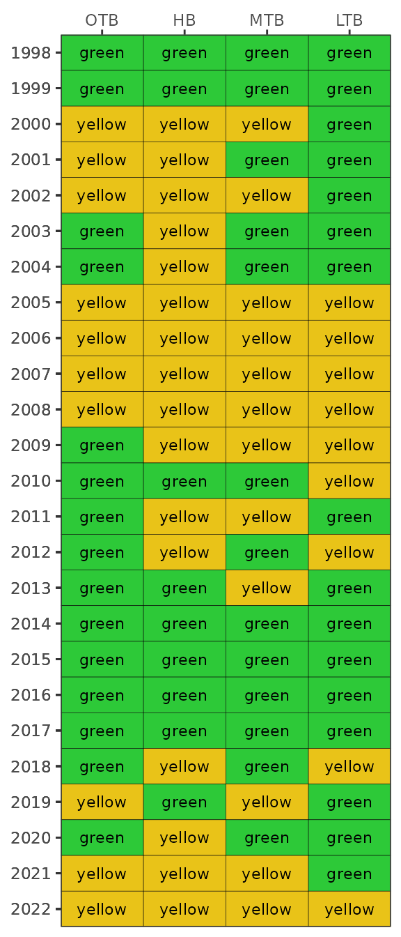
Each of the plots can also be produced as plotly interactive plots by setting
plotly = TRUE inside each function.
show_tbniscr(tbniscr, plotly = T)
show_tbniscrall(tbniscr, plotly = T)
show_tbnimatrix(tbniscr, plotly = T)The breakpoints for the categorical outcomes of the TBNI scores shown
by the colors in each graph are based on the 33rd and 50th percentiles
of the distribution of all TBNI scores calculated for Tampa Bay. This
plotting option is provided for consistency with existing TBEP reporting
tools, e.g., the water quality report
card returned by show_matrix(). The categorical
outcomes serve as management guidelines each year for activities to
support environmental resources of the Bay: Stay the Course, Caution, and On Alert [3].
The graphs returned by the plotting functions are ggplot
objects that can be further modified. They can be combined below using
patchwork in a
single graphic showing the trends over time as both categorical outcomes
in the matrix and continuous scores in the bottom plot.
p1 <- show_tbnimatrix(tbniscr, txtsz = NULL, rev = TRUE, position = 'bottom') +
  scale_y_continuous(expand = c(0,0), breaks = c(1998:2020)) +
  coord_flip() +
  theme(axis.text.x = element_blank())

p2 <- show_tbniscr(tbniscr)

p1 + p2 + plot_layout(ncol = 1, heights = c(0.3, 1))