Each year, TBEP partners collect seagrass transect data at fixed locations in Tampa Bay. Data have been collected since the mid 1990s and are hosted online at the Tampa Bay Water Atlas by the University of South Florida Water Institute. Functions are available in tbeptools for downloading, analyzing, and plotting these data.
Data import and included datasets
There are two datasets included in tbeptools that show the actively
monitored transect locations in Tampa Bay. The trnpts
dataset is a point object for the starting location of each transect and
the trnlns dataset is a line object showing the approximate
direction and length of each transect beginning at each point in
trnpts. Each dataset also includes the
MonAgency column that indicates which monitoring agency
collects the data at each transect.
trnpts
#> Simple feature collection with 66 features and 11 fields
#> Geometry type: POINT
#> Dimension:     XY
#> Bounding box:  xmin: -82.8089 ymin: 27.49925 xmax: -82.39305 ymax: 28.0001
#> Geodetic CRS:  WGS 84
#> First 10 features:
#>    SEGMENT TRANSECT TRAN_ID Metermark    ID   LAT_DD   LONG_DD MonAgency STATUS
#> 1        1        1    S1T1         0 START 27.99498 -82.68325     EPCHC ACTIVE
#> 2        1        3    S1T3         0 START 28.00010 -82.66417     EPCHC ACTIVE
#> 3        1        5    S1T5         0 START 27.95788 -82.54663      FDEP ACTIVE
#> 4        1        6    S1T6         0 START 27.91348 -82.53282     EPCHC ACTIVE
#> 5        1        8    S1T8         0 START 27.86233 -82.56867     EPCHC ACTIVE
#> 6        1       13   S1T13         0 START 27.92428 -82.70232     EPCHC ACTIVE
#> 7        1       14   S1T14         0 START 27.85533 -82.59738     EPCHC ACTIVE
#> 8        1       15   S1T15         0 START 27.87408 -82.53098     EPCHC ACTIVE
#> 9        1       16   S1T16         0 START 27.88228 -82.62015     PCDEM ACTIVE
#> 10       1       17   S1T17         0 START 27.90498 -82.64793     PCDEM ACTIVE
#>    Comments bay_segment                   geometry
#> 1      <NA>         OTB POINT (-82.68325 27.99498)
#> 2      <NA>         OTB  POINT (-82.66417 28.0001)
#> 3      <NA>         OTB POINT (-82.54663 27.95788)
#> 4      <NA>         OTB POINT (-82.53282 27.91348)
#> 5      <NA>         OTB POINT (-82.56867 27.86233)
#> 6      <NA>         OTB POINT (-82.70232 27.92428)
#> 7      <NA>         OTB POINT (-82.59738 27.85533)
#> 8      <NA>         OTB POINT (-82.53098 27.87408)
#> 9      <NA>         OTB POINT (-82.62015 27.88228)
#> 10     <NA>         OTB POINT (-82.64793 27.90498)
trnlns
#> Simple feature collection with 66 features and 8 fields
#> Geometry type: LINESTRING
#> Dimension:     XYM
#> Bounding box:  xmin: -82.8118 ymin: 27.49807 xmax: -82.39306 ymax: 28.0001
#> m_range:       mmin: 0 mmax: 2700
#> Geodetic CRS:  WGS 84
#> First 10 features:
#>    OBJECTID  Site Shape_Leng MonAgency ActiveYN Comments     bearing
#> 1         1  S1T1   300.1400     EPCHC      YES     <NA>  116.533756
#> 2         5 S1T13  1102.6182     EPCHC      YES     <NA>   -4.689701
#> 3         6 S1T14   800.4500     EPCHC      YES     <NA>  109.402541
#> 4         7 S1T15   701.0075     EPCHC      YES     <NA>  -85.765142
#> 5         8 S1T16   998.9961     PCDEM      YES     <NA>   13.913960
#> 6         9 S1T17  2698.5773     PCDEM      YES     <NA>  -21.165576
#> 7        10 S1T18   997.5451     EPCHC      YES     <NA> -123.050914
#> 8        12  S1T3   401.5991     EPCHC      YES     <NA> -128.034327
#> 9        14  S1T5   457.5927      FDEP      YES     <NA> -121.861907
#> 10       15  S1T6   398.6606     EPCHC      YES     <NA>  -89.362036
#>    bay_segment                       geometry
#> 1          OTB LINESTRING M (-82.68325 27....
#> 2          OTB LINESTRING M (-82.70232 27....
#> 3          OTB LINESTRING M (-82.59738 27....
#> 4          OTB LINESTRING M (-82.53098 27....
#> 5          OTB LINESTRING M (-82.62015 27....
#> 6          OTB LINESTRING M (-82.64791 27....
#> 7          OTB LINESTRING M (-82.61143 27....
#> 8          OTB LINESTRING M (-82.66417 28....
#> 9          OTB LINESTRING M (-82.54663 27....
#> 10         OTB LINESTRING M (-82.53282 27....
The two datasets are sf() (simple features) objects and
are easily mapped with mapview() to view their
locations.
cols <- c("#E16A86", "#CB7F2F", "#9F9400", "#50A315", "#00AC79", "#00AAB7", "#009ADE", "#A87BE4", "#DA65C3")

mapview(trnpts, zcol = 'MonAgency', lwd = 0, legend = F, homebutton = F, col.regions = cols) +
  mapview(trnlns, zcol = 'MonAgency', homebutton = F, layer.name = 'Monitoring Agency', lwd = 4, color = cols)
The transect data can be downloaded from the Water Atlas using the
read_transect() function. The only required argument for
this function is training, which indicates if you want to
download training data or the complete dataset, i.e.,
training = TRUE or training = FALSE (default).
In the former case, a small dataset is downloaded that includes only
data collected during an annual training event. These are primarily used
internally by TBEP staff to assess precision among different training
crews. The data are downloaded as a JSON object and formatted internally
using the read_formtransect() function. Shoot density is
reported as number of shoots per square meter and is corrected for the
quadrat size entered in the raw data. Abundance is reported as a numeric
value from 0 -5 for Braun-Blanquet coverage estimates and blade length
is in cm.
# import training data
traindat <- read_transect(training = TRUE)

# view the data
traindat
#> # A tibble: 2,103 × 11
#>       yr grp   grpact    Crew  MonitoringAgency Site  Depth Species var   aveval
#>    <int> <chr> <chr>     <chr> <chr>            <chr> <int> <chr>   <chr>  <dbl>
#>  1  2020 A     2020: MC… K. H… MCNRD            1       -50 Halodu… Abun…    3
#>  2  2020 A     2020: MC… K. H… MCNRD            1       -50 Halodu… Blad…    0
#>  3  2020 A     2020: MC… K. H… MCNRD            1       -50 Halodu… Shor…    0
#>  4  2020 A     2020: MC… K. H… MCNRD            2       -40 No Cov… Abun…    0
#>  5  2020 A     2020: MC… K. H… MCNRD            2       -40 No Cov… Blad…    0
#>  6  2020 A     2020: MC… K. H… MCNRD            2       -40 No Cov… Shor…    0
#>  7  2020 A     2020: MC… K. H… MCNRD            3       -60 Halodu… Abun…    5
#>  8  2020 A     2020: MC… K. H… MCNRD            3       -60 Halodu… Blad…   22
#>  9  2020 A     2020: MC… K. H… MCNRD            3       -60 Halodu… Shor…   27.3
#> 10  2020 A     2020: MC… K. H… MCNRD            3       -60 Thalas… Abun…    1
#> # ℹ 2,093 more rows
#> # ℹ 1 more variable: sdval <dbl>
Change the training argument to FALSE to
download the entire transect database. This may take a few seconds.
# import entire transct dataset as JSON
transect <- read_transect(training = FALSE)

# view the data
transect
#> # A tibble: 164,724 × 11
#>    Crew              MonitoringAgency Date       Transect Site  Depth Savspecies
#>    <chr>             <chr>            <date>     <chr>    <chr> <int> <chr>
#>  1 A. McClory, A. I… MCNRD            2024-08-13 S4T2     0       -10 No Cover
#>  2 A. McClory, A. I… MCNRD            2024-08-13 S4T2     0       -10 No Cover
#>  3 A. McClory, A. I… MCNRD            2024-08-13 S4T2     0       -10 No Cover
#>  4 A. McClory, A. I… MCNRD            2024-08-13 S4T2     100     -40 Thalassia
#>  5 A. McClory, A. I… MCNRD            2024-08-13 S4T2     100     -40 Thalassia
#>  6 A. McClory, A. I… MCNRD            2024-08-13 S4T2     100     -40 Thalassia
#>  7 A. McClory, A. I… MCNRD            2024-08-13 S4T2     125     -25 Thalassia
#>  8 A. McClory, A. I… MCNRD            2024-08-13 S4T2     125     -25 Thalassia
#>  9 A. McClory, A. I… MCNRD            2024-08-13 S4T2     125     -25 Thalassia
#> 10 A. McClory, A. I… MCNRD            2024-08-13 S4T2     150      -5 Halodule
#> # ℹ 164,714 more rows
#> # ℹ 4 more variables: SeagrassEdge <dbl>, var <chr>, aveval <dbl>, sdval <dbl>
The columns in the complete transect database describe the crew
(Crew), the monitoring agency
(MonitoringAgency), sample date (Date),
transect name (Transect), the meter location for the
quadrat along the transect (Site, m), depth at the site
(Depth, cm), Seagrass species (Savspecies),
distance of the seagrass edge on the transect
(SeagrassEdge, m), the seagrass variable
(var), average value of the variable (aveval),
and standard deviation of the variable if appropriate
(sdval).
If the raw, unformatted transect data are preferred, use the
raw = TRUE argument for read_transect().
# raw transect data
transectraw <- read_transect(training = FALSE, raw = TRUE)

# view the data
transectraw
#> # A tibble: 55,224 × 46
#>    IDall AssessmentYear CreatedAt   Crew  CountingTech SeagrassEdge Secchi Sonde
#>    <int>          <int> <chr>       <chr> <chr>               <dbl>  <dbl> <lgl>
#>  1     2           1998 1998-10-15… NA    NA                     NA     NA FALSE
#>  2     2           1998 1998-10-15… NA    NA                     NA     NA FALSE
#>  3     2           1998 1998-10-15… NA    NA                     NA     NA FALSE
#>  4     2           1998 1998-10-15… NA    NA                     NA     NA FALSE
#>  5     2           1998 1998-10-15… NA    NA                     NA     NA FALSE
#>  6     2           1998 1998-10-15… NA    NA                     NA     NA FALSE
#>  7     2           1998 1998-10-15… NA    NA                     NA     NA FALSE
#>  8     2           1998 1998-10-15… NA    NA                     NA     NA FALSE
#>  9     2           1998 1998-10-15… NA    NA                     NA     NA FALSE
#> 10     2           1998 1998-10-15… NA    NA                     NA     NA FALSE
#> # ℹ 55,214 more rows
#> # ℹ 38 more variables: Weather <chr>, Hidden <lgl>, HiddenReason <lgl>,
#> #   IsComplete <lgl>, QASubmittedAt <chr>, ReadyForQA <lgl>,
#> #   QACompletedAt <chr>, MonitoringAgency <chr>, Transect <chr>,
#> #   BaySegment <chr>, ID <int>, ObservationDate <chr>, Site <int>,
#> #   Species <chr>, SpeciesAbundance <chr>, Appearance <chr>,
#> #   BladeLength_1 <int>, BladeLength_2 <int>, BladeLength_3 <int>, …
Calculating seagrass frequency occurrence
The rest of the seagrass functions in tbeptools were developed to
work with the complete database. Only the show_complot()
function (see below) was developed for the training data. The rest of
the functions can be used to estimate and plot frequency occurrence
data.
The anlz_transectocc() function summarizes frequency
occurrence for all transects and dates by collapsing species results
across quadrats within each transect. Abundance and frequency occurrence
are estimated as in Sherwood et al. 2017, equations 1 and 2 [1]. In short, frequency occurrence is estimated
as the number of instances a species was observed along a transect
divided by the number of placements along a transect and average
abundance was estimated as the sum of species-specific Braun-Blanquet
scores divided by the number of placements along a transect. The
estimates are obtained for all seagrass species, including Caulerpa spp.
(attached macroalgae), Dapis (cyanobacteria), and Chaetomorpha (drift
green algae), whereas all attached and drift algae species are
aggregated. Drift or attached macroalgae and cyanobacteria (Dapis)
estimates may not be accurate prior to 2021.
transectocc <- anlz_transectocc(transect)
transectocc
#> # A tibble: 41,916 × 6
#> # Groups:   Date, Transect [1,497]
#>    Date       Transect Savspecies                  nsites foest bbest
#>    <date>     <chr>    <chr>                        <int> <dbl> <dbl>
#>  1 1997-10-11 S2T3     "AA"                            41     0     0
#>  2 1997-10-11 S2T3     "Caulerpa"                      41     0     0
#>  3 1997-10-11 S2T3     "Chaetomorpha"                  41     0     0
#>  4 1997-10-11 S2T3     "DA"                            41     0     0
#>  5 1997-10-11 S2T3     "DB: Dictyota\r\n"              41     0     0
#>  6 1997-10-11 S2T3     "DB: Drift Brown\r\n"           41     0     0
#>  7 1997-10-11 S2T3     "DG: Drift Green"               41     0     0
#>  8 1997-10-11 S2T3     "DG: Ulva"                      41     0     0
#>  9 1997-10-11 S2T3     "DG: Ulva fasciata\r\n"         41     0     0
#> 10 1997-10-11 S2T3     "DG: Ulva intestinales\r\n"     41     0     0
#> # ℹ 41,906 more rows
The second function, anlz_transectave(), takes the
results from anlz_transectocc() and estimates annual
results across major bay segments for all seagrass species by averaging
frequency occurrence across transects. This function is used internally
within the show_transectmatrix() function to create summary
plots. The frequency occurrence estimates are also binned into
categories for simple trend assessments, e.g., red < 25%, orange
25-50%, yellow 50-75%, and green > 75%. Results for specific bay
segments and annual ranges can be filtered with the
bay_segment and yrrng arguments.
transectave <- anlz_transectave(transectocc)
transectave
#> # A tibble: 168 × 4
#> # Groups:   bay_segment [6]
#>    bay_segment    yr foest focat
#>    <fct>       <dbl> <dbl> <fct>
#>  1 All          1998  58.0 #E9C318
#>  2 OTB          1998  65.5 #E9C318
#>  3 HB           1998  15.0 #CC3231
#>  4 MTB          1998  53.7 #E9C318
#>  5 LTB          1998  80.8 #2DC938
#>  6 BCB          1998  81.0 #2DC938
#>  7 All          1999  51.4 #E9C318
#>  8 OTB          1999  64.7 #E9C318
#>  9 HB           1999  10.1 #CC3231
#> 10 MTB          1999  51.8 #E9C318
#> # ℹ 158 more rows
The third function, anlz_transectavespp(), takes the
results from anlz_transectocc() and estimates annual
averages across major bay segments as in the last function, but results
are retained for individual species. This function is used internally
within the show_transectavespp() function to create summary
plots. All summaries are aggregated across the selected bay segments,
i.e., the default is to average by species/year across all segments.
Results for an individual bay segment can be returned with the
appropriate argument, e.g., by using bay_segment = 'OTB' to
select only Old Tampa Bay. Results can also be filtered by specific
species using the species argument, where the default is to
return all. Caulerpa spp., Dapis spp., and
Chaetomorpha spp. are also included.
transectavespp <- anlz_transectavespp(transectocc)
transectavespp
#> # A tibble: 252 × 3
#>       yr Savspecies    foest
#>    <dbl> <fct>         <dbl>
#>  1  1998 Caulerpa     0.0166
#>  2  1998 Chaetomorpha 0
#>  3  1998 Dapis        0
#>  4  1998 Halodule     0.361
#>  5  1998 Halophila    0
#>  6  1998 Ruppia       0.0112
#>  7  1998 Syringodium  0.0451
#>  8  1998 Thalassia    0.254
#>  9  1998 total        0.580
#> 10  1999 Caulerpa     0.0283
#> # ℹ 242 more rows
Results for individual bay segments from
anlz_transectavespp() can be retained by setting the
by_seg argument to TRUE. Note that totals are
not returned in this case.
transectavespp <- anlz_transectavespp(transectocc, by_seg = TRUE)
transectavespp
#> # A tibble: 1,400 × 5
#>       yr bay_segment Savspecies   foest nsites
#>    <dbl> <fct>       <fct>        <dbl>  <int>
#>  1  1998 BCB         Caulerpa     0         96
#>  2  1998 BCB         Chaetomorpha 0         96
#>  3  1998 BCB         Dapis        0         96
#>  4  1998 BCB         Halodule     0.613     96
#>  5  1998 BCB         Halophila    0         96
#>  6  1998 BCB         No Cover     0.190     96
#>  7  1998 BCB         Ruppia       0         96
#>  8  1998 BCB         Syringodium  0         96
#>  9  1998 BCB         Thalassia    0.304     96
#> 10  1998 BCB         total        0.810     96
#> # ℹ 1,390 more rows
Plotting results
There is one plotting function for the training data. The
show_compplot() function is used to compare training data
between crews for a selected species (species argument) and
variable (varplo argument).
show_compplot(traindat, yr = 2025, site = '3', species = 'Halodule', varplo = 'Abundance', base_size = 14)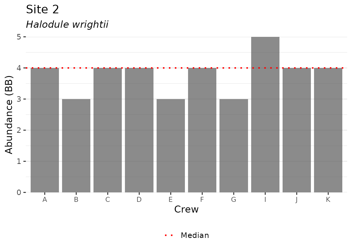
The rest of the plotting functions work with the complete transect
data. Data for an individual transect can be viewed with the
show_transect() function by entering the transect (site)
number, species (one to many), and variable to plot. The plot shows
relative values for the selected species and variable by distance along
the transect (x-axis) and year of sampling (y-axis). The plots provide
an overall summary of temporal and spatial changes in the selected
seagrass metric for an individual location.
show_transect(transect, site = 'S3T10', species = 'Halodule', varplo = 'Abundance')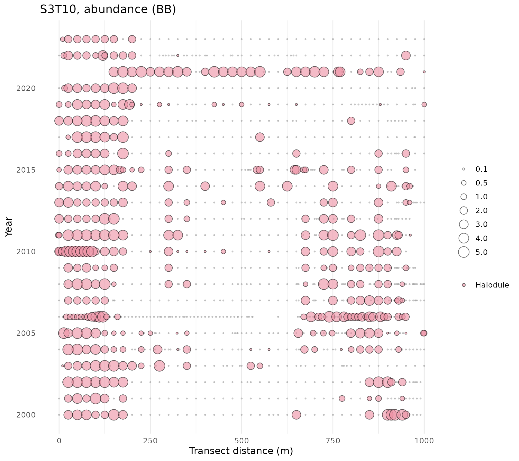
The plot can also be produced as a plotly interactive plot by setting
plotly = TRUE inside the function. Note that the size
legend is merged with the species legend, where the point size is the
average abundance for the species. The sizes can be viewed on mouseover
of each point.
show_transect(transect, site = 'S3T10', species = 'Halodule', varplo = 'Abundance', plotly = T)The show_transect() function can also be used to plot
multiple species. One to many species can be provided to the
species argument.
show_transect(transect, site = 'S3T10', species = c('Halodule', 'Syringodium', 'Thalassia'), varplo = 'Abundance')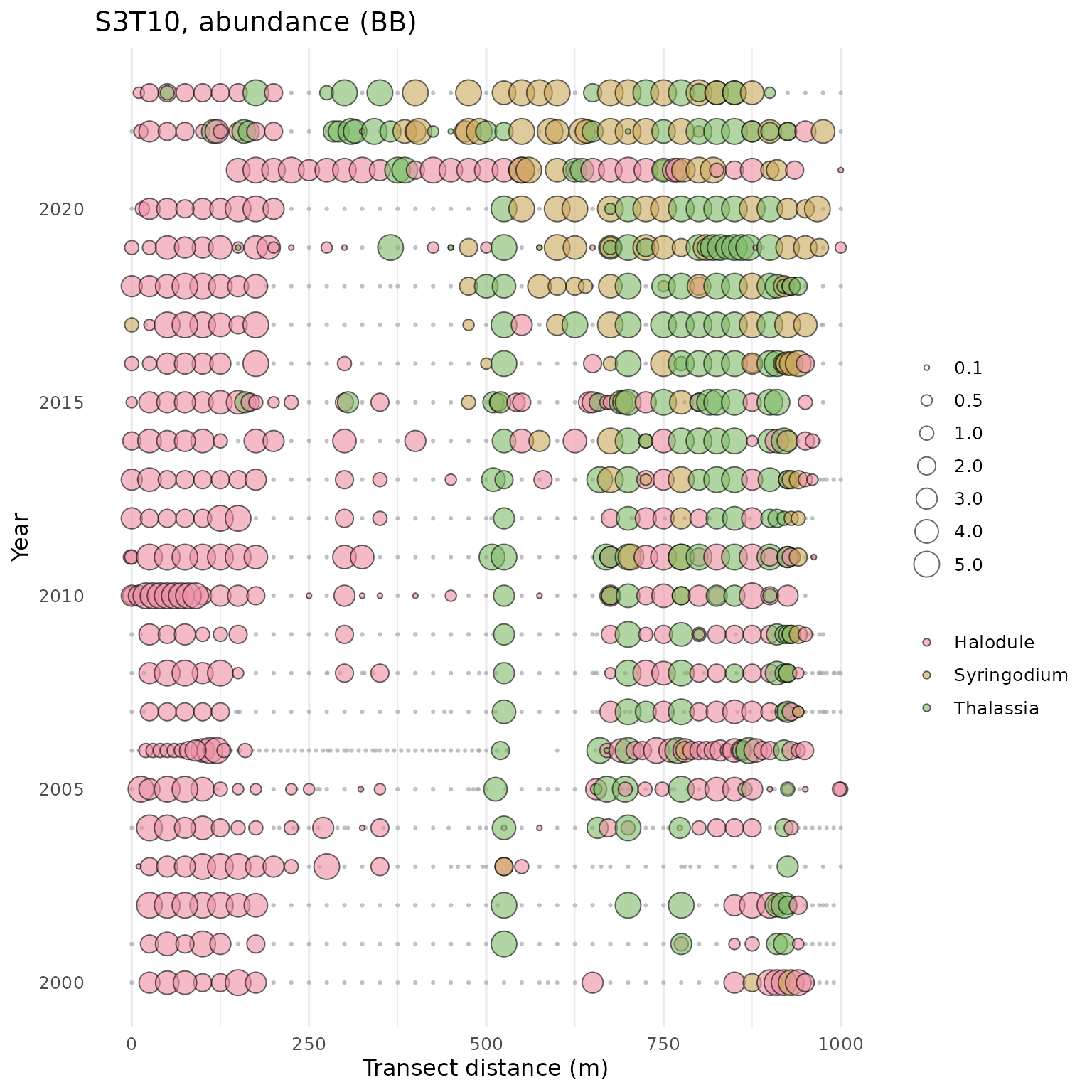
The plots can also be separated into facets for each species using
facet = TRUE. This is useful to reduce overplotting of
multiple species found at the same location.
show_transect(transect, site = 'S3T10', species = c('Halodule', 'Syringodium', 'Thalassia'), varplo = 'Abundance', facet = TRUE)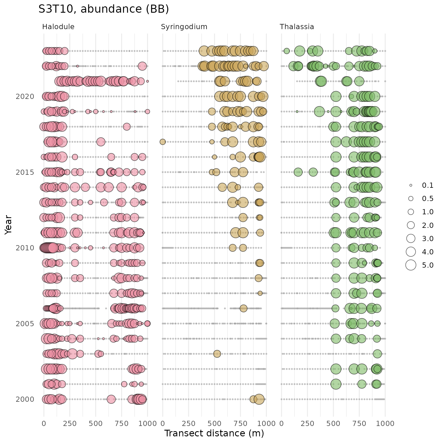
The show_transectsum() function provides an alternative
summary of data at an individual transect. This plot provides a quick
visual assessment of how frequency occurrence or abundance for multiple
species has changed over time at a selected transect. Unlike
show_transect(), the plot shows aggregated results across
quadrats along the transect and uses summarized data from the
anlz_transectocc() function as input.
show_transectsum(transectocc, site = 'S3T10')A summary matrix of frequency occurrence estimates across all species
can be plotted with show_transectmatrix(). This uses
results from the anlz_transectocc() and
anlz_transectave() functions to estimate annual averages by
bay segment. The continuous frequency occurrence estimates are binned
into color categories described above, as in Table 1 in [2].
show_transectmatrix(transectocc)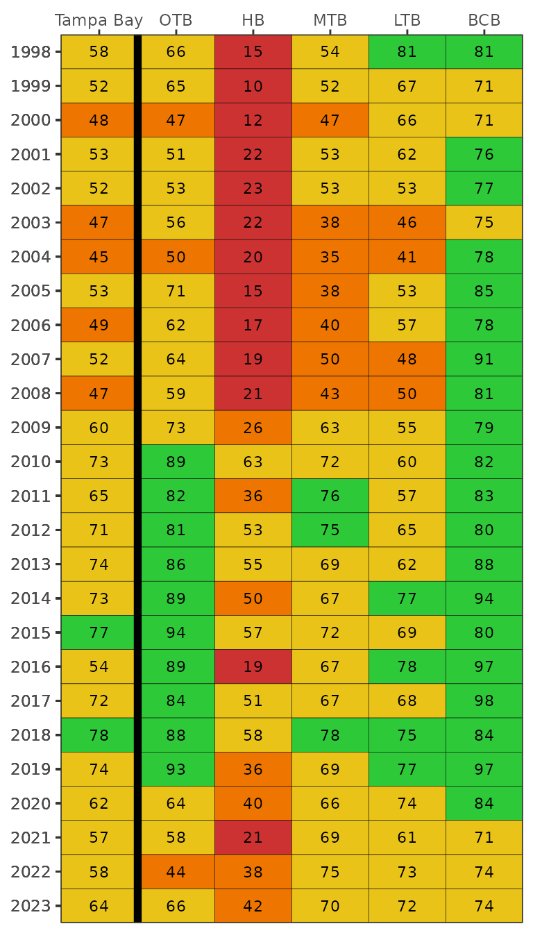
The default color scheme is based on arbitrary breaks at 25, 50, and
75 percent frequency occurrence. These don’t necessarily translate to
any ecological breakpoints. Use neutral = TRUE to use a
neutral and continuous color palette.
show_transectmatrix(transectocc, neutral = T)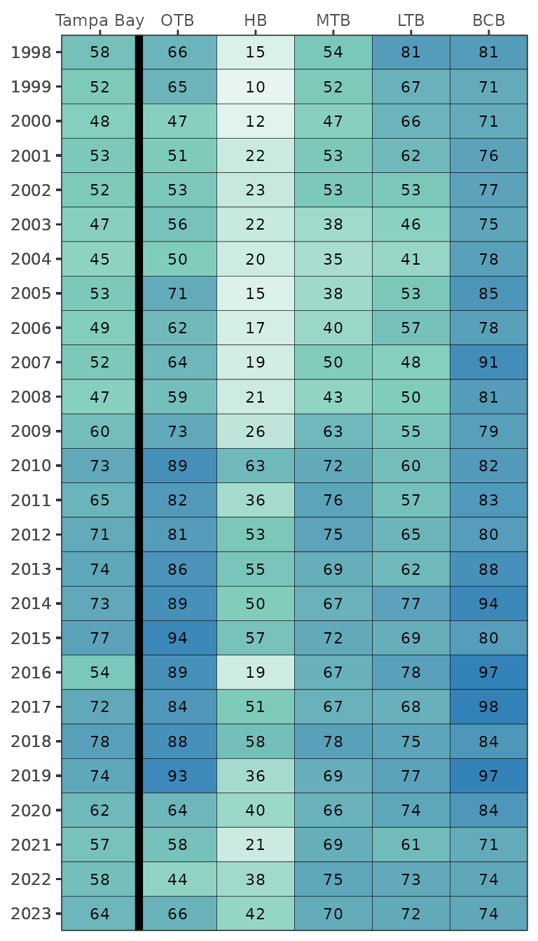
The matrix can also be produced as a plotly interactive plot by setting
plotly = TRUE inside the function.
show_transectmatrix(transectocc, plotly = T)Time series plots of annual averages of frequency occurrence
estimates by each species can be shown with the
show_transectavespp() function. By default, all estimates
are averaged across all bay segments for each species. The plot is a
representation of Figure 2 in [2].
show_transectavespp(transectocc)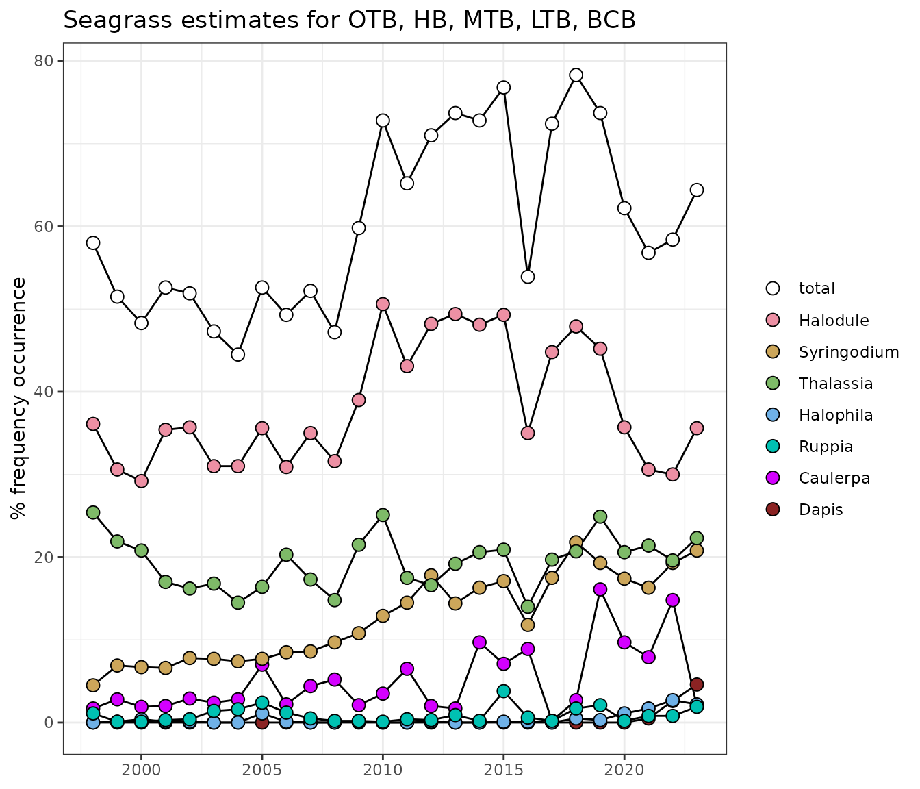
Results for individual segments and species can be returned with the
bay_segment and species arguments. Use the
argument total = FALSE to omit the total frequency
occurrence from the plot.
show_transectavespp(transectocc, bay_segment = 'LTB', species = c('Syringodium', 'Thalassia'), total = FALSE)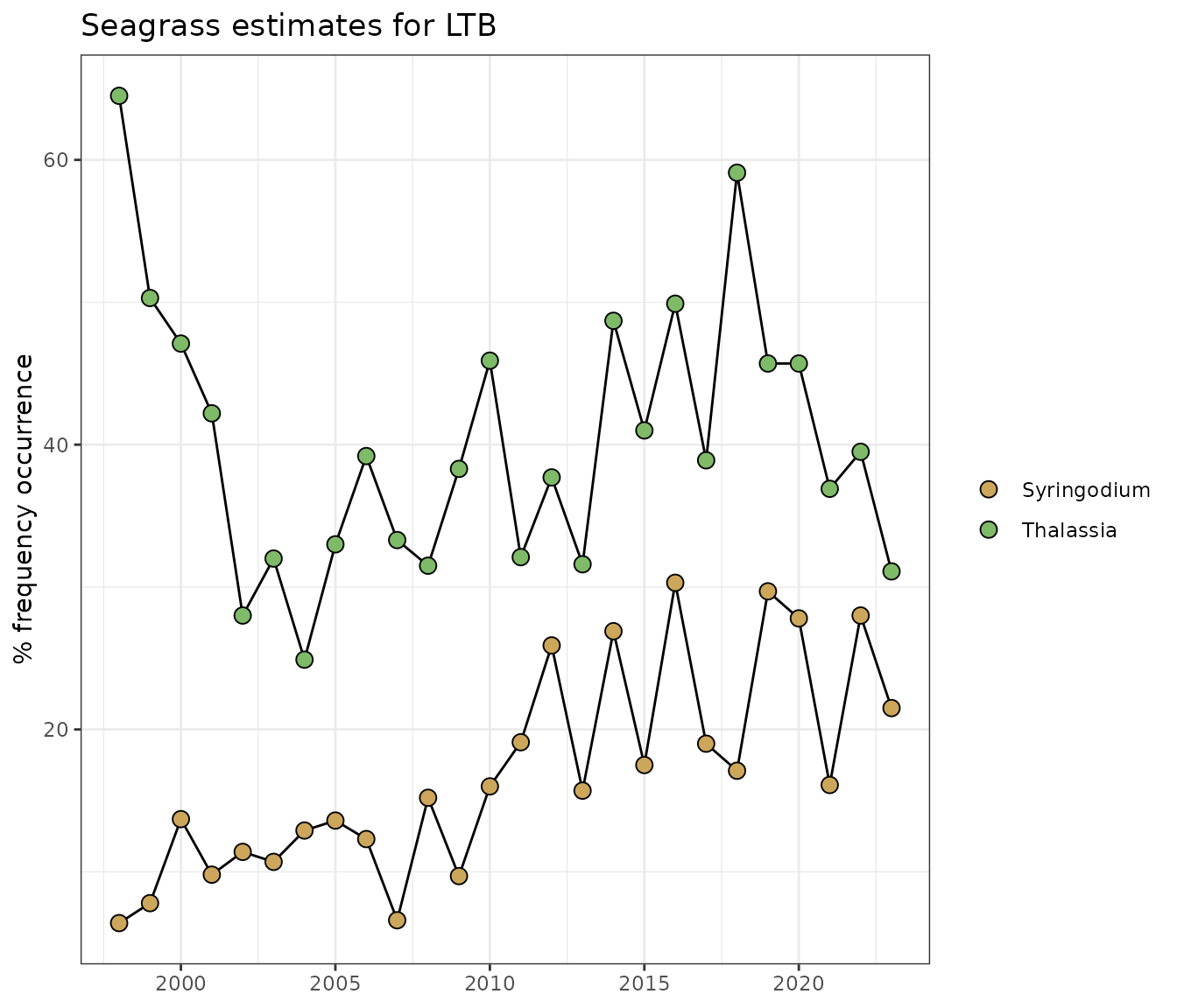
The plot can also be produced as a plotly interactive plot by setting
plotly = TRUE inside the function.
show_transectavespp(transectocc, bay_segment = 'LTB', species = c('Syringodium', 'Thalassia'), plotly = T)As an alternative to plotting the species averages over time with
show_transectavespp(), a table can be created by setting
asreact = TRUE. Filtering options that apply to the plot
also apply to the table, e.g., filtering by the four major bay segments
and specific year ranges. Also note that the totals are not returned in
the table.
show_transectavespp(transectocc, asreact = T, bay_segment = c('HB', 'OTB', 'MTB', 'LTB'), yrrng = c(2006, 2012))All of the above describes methods in tbeptools for working with
transect monitoring data. Seagrass coverage maps are also created
approximately biennially by the Southwest Florida Water Management
District, available at https://data-swfwmd.opendata.arcgis.com/.
The seagrass data object included with the package shows
Tampa Bay coverage total for each year of available data, including a
1950s reference estimate. The show_seagrasscoverage()
function creates the flagship seagrass coverage graphic to report on
changes over time from these data.
show_seagrasscoverage(seagrass)