Tampa Bay Benthic Index (TBBI)
Background
The Tampa Bay Benthic Index (TBBI) [1,2]) is an assessment method that quantifies the ecological health of the benthic community in Tampa Bay. The index provides a complementary approach to evaluating environmental condition that is supported by other assessment methods currently available for the region (e.g., water quality report card, nekton index, etc.). The tbeptools package includes several functions described below to import data required for the index and plot the results to view trends over time. Each of the functions are described in detail below.
The TBBI uses data from the Tampa Bay Benthic Monitoring Program as part of the Environmental Protection Commission (EPC) of Hillsborough Country. The data are updated annually on a public site maintained by EPC, typically in December after Summer/Fall sampling. This is the same website that hosts water quality data used for the water quality report card. The required data for the TBBI are more extensive than the water quality report card and the data are made available as a zipped folder of csv files, available here. The process for downloading and working with the data are similar as for the other functions in tbeptools.
Data import and included datasets
Data for calculating TBBI scores can be imported into the current R
session using the read_importbenthic() function. This
function downloads the zipped folder of base tables used for the TBBI
from the EPC site if the data have not already been downloaded to the
location specified by the input arguments.
To download the data with tbeptools, first create a character path
for the location where you want to download the zipped files. If one
does not exist, specify a location and name for the downloaded file.
Here, we name the folder benthic.zip and download it on our
desktop.
path <- '~/Desktop/benthic.zip'
benthicdata <- read_importbenthic(path)
Running the above code will return the following error:
#> Error in read_importbenthic() : File at path does not exist, use download_latest = TRUEWe get an error message from the function indicating that the file is
not found. This makes sense because the file does not exist yet, so we
need to tell the function to download the latest file. This is done by
changing the download_latest argument to TRUE
(the default is FALSE).
benthicdata <- read_importbenthic(path, download_latest = T)
#> File ~/Desktop/benthic.zip does not exist, replacing with downloaded file...Now we get an indication that the file on the server is being
downloaded. When the download is complete, we’ll have the data
downloaded and saved to the benthicdata object in the
current R session.
If we try to run the function again after downloading the data, we get the following message. This check is done to make sure that the data are not unnecessarily downloaded if the current file matches the file on the server.
benthicdata <- read_importbenthic(path, download_latest = T)
#> File is current..Every time that tbeptools is used to work with the benthic data,
read_importbenthic() should be used to import the data. You
will always receive the message File is current... if your
local file matches the one on the server. However, data are periodically
updated and posted on the server. If download_latest = TRUE
and your local file is out of date, you will receive the following
message:
#> Replacing local file with current...Calculating TBBI scores
After the data are imported, you can view them from the assigned object. The data are provided as a nested tibble that includes three different datasets: station information, field sample data (salinity), and detailed taxa information.
benthicdata
#> # A tibble: 3 × 2
#>   name         value
#>   <chr>        <list>
#> 1 stations     <tibble [4,915 × 10]>
#> 2 fieldsamples <tibble [5,334 × 3]>
#> 3 taxacounts   <tibble [153,895 × 7]>
The individual datasets can be viewed by extracting them from the
parent object using the deframe() function from the tibble
package.
# see all
deframe(benthicdata)
#> $stations
#> # A tibble: 4,915 × 10
#>    StationID StationNumber AreaAbbr FundingProject ProgramID ProgramName
#>        <int> <chr>         <chr>    <chr>              <int> <chr>
#>  1       448 02BBs301      MTB      Apollo Beach           4 Benthic Monitoring
#>  2       449 02BBs305      MTB      Apollo Beach           4 Benthic Monitoring
#>  3       450 02BBs307      MTB      Apollo Beach           4 Benthic Monitoring
#>  4       451 02BBs364      MTB      Apollo Beach           4 Benthic Monitoring
#>  5       452 02BBs369      MTB      Apollo Beach           4 Benthic Monitoring
#>  6       453 02BBs395      MTB      Apollo Beach           4 Benthic Monitoring
#>  7       454 02BBs397      MTB      Apollo Beach           4 Benthic Monitoring
#>  8       455 02BBs398      MTB      Apollo Beach           4 Benthic Monitoring
#>  9       456 02BBs401      MTB      Apollo Beach           4 Benthic Monitoring
#> 10       457 02BBs402      MTB      Apollo Beach           4 Benthic Monitoring
#> # ℹ 4,905 more rows
#> # ℹ 4 more variables: Latitude <dbl>, Longitude <dbl>, date <date>, yr <dbl>
#>
#> $fieldsamples
#> # A tibble: 5,334 × 3
#>    StationID date       Salinity
#>        <int> <date>        <dbl>
#>  1       448 2002-05-21     30.5
#>  2       449 2002-05-20     30.8
#>  3       450 2002-05-21     30.5
#>  4       451 2002-05-21     30.6
#>  5       452 2002-05-20     30
#>  6       453 2002-05-21     30.6
#>  7       454 2002-05-21     30.5
#>  8       455 2002-05-21     30.3
#>  9       456 2002-05-20     30.0
#> 10       457 2002-05-20     29.9
#> # ℹ 5,324 more rows
#>
#> $taxacounts
#> # A tibble: 153,895 × 7
#>    StationID TaxaCountID TaxaListID FAMILY           NAME     TaxaCount AdjCount
#>        <int>       <int>      <int> <chr>            <chr>        <dbl>    <dbl>
#>  1     11321      152055       1198 Anomiidae        Anomia …         1       25
#>  2     11321      152056       1224 Carditidae       Cardite…         1       25
#>  3       584      233277        624 Cirratulidae     Chaetoz…         1       25
#>  4     11321      152057       1306 Veneridae        Chione …         3       75
#>  5      3132      239443        352 Pilargidae       Sigambr…        14      350
#>  6     11321      152058       1088 Pyramidellidae   Turboni…         6      150
#>  7      2541      140530        258 NULL             NEMERTEA         8      200
#>  8      2542      140531        258 NULL             NEMERTEA         2       50
#>  9      2992      140631        262 NULL             Palaeon…         4      100
#> 10      3003      140635        285 Tetrastemmatidae Tetrast…         2       50
#> # ℹ 153,885 more rows

# get only station dat
deframe(benthicdata)[['stations']]
#> # A tibble: 4,915 × 10
#>    StationID StationNumber AreaAbbr FundingProject ProgramID ProgramName
#>        <int> <chr>         <chr>    <chr>              <int> <chr>
#>  1       448 02BBs301      MTB      Apollo Beach           4 Benthic Monitoring
#>  2       449 02BBs305      MTB      Apollo Beach           4 Benthic Monitoring
#>  3       450 02BBs307      MTB      Apollo Beach           4 Benthic Monitoring
#>  4       451 02BBs364      MTB      Apollo Beach           4 Benthic Monitoring
#>  5       452 02BBs369      MTB      Apollo Beach           4 Benthic Monitoring
#>  6       453 02BBs395      MTB      Apollo Beach           4 Benthic Monitoring
#>  7       454 02BBs397      MTB      Apollo Beach           4 Benthic Monitoring
#>  8       455 02BBs398      MTB      Apollo Beach           4 Benthic Monitoring
#>  9       456 02BBs401      MTB      Apollo Beach           4 Benthic Monitoring
#> 10       457 02BBs402      MTB      Apollo Beach           4 Benthic Monitoring
#> # ℹ 4,905 more rows
#> # ℹ 4 more variables: Latitude <dbl>, Longitude <dbl>, date <date>, yr <dbl>
The anlz_tbbiscr() function uses the nested
benthicdata to estimate the TBBI scores at each site. The
TBBI scores typically range from 0 to 100 and are grouped into
categories that describe the general condition of the benthic community.
Scores less than 73 are considered “degraded”, scores between 73 and 87
are “intermediate”, and scores greater than 87 are “healthy”. Locations
that were sampled but no organisms were found are assigned a score of
zero and a category of “empty sample”. The total abundance
(TotalAbundance, organisms/m2), species richness
(SpeciesRichness) and bottom salinity
(Salinity, psu) are also provided. Some metrics for the
TBBI are corrected for salinity and bottom measurements taken at the
time of sampling are required for accurate calculation of the TBBI.
tbbiscr <- anlz_tbbiscr(benthicdata)
tbbiscr
#> # A tibble: 4,915 × 15
#>    StationID StationNumber AreaAbbr FundingProject ProgramID ProgramName
#>        <int> <chr>         <chr>    <chr>              <int> <chr>
#>  1       448 02BBs301      MTB      Apollo Beach           4 Benthic Monitoring
#>  2       449 02BBs305      MTB      Apollo Beach           4 Benthic Monitoring
#>  3       450 02BBs307      MTB      Apollo Beach           4 Benthic Monitoring
#>  4       451 02BBs364      MTB      Apollo Beach           4 Benthic Monitoring
#>  5       452 02BBs369      MTB      Apollo Beach           4 Benthic Monitoring
#>  6       453 02BBs395      MTB      Apollo Beach           4 Benthic Monitoring
#>  7       454 02BBs397      MTB      Apollo Beach           4 Benthic Monitoring
#>  8       455 02BBs398      MTB      Apollo Beach           4 Benthic Monitoring
#>  9       456 02BBs401      MTB      Apollo Beach           4 Benthic Monitoring
#> 10       457 02BBs402      MTB      Apollo Beach           4 Benthic Monitoring
#> # ℹ 4,905 more rows
#> # ℹ 9 more variables: Latitude <dbl>, Longitude <dbl>, date <date>, yr <dbl>,
#> #   TotalAbundance <dbl>, SpeciesRichness <dbl>, TBBI <dbl>, TBBICat <chr>,
#> #   Salinity <dbl>
Plotting results
The TBBI scores can be viewed as annual averages for each bay segment
using the show_tbbimatrix() function. The
show_tbbimatrix() plots the annual bay segment averages as
categorical values in a conventional “stoplight” graphic. A baywide
estimate is also returned, one based on all samples across all locations
(“All”) and another weighted by the relative surface areas of each bay
segment (“All (wt)”). The input to show_tbbimatrix()
function is the output from the anlz_tbbiscr()
function.
show_tbbimatrix(tbbiscr)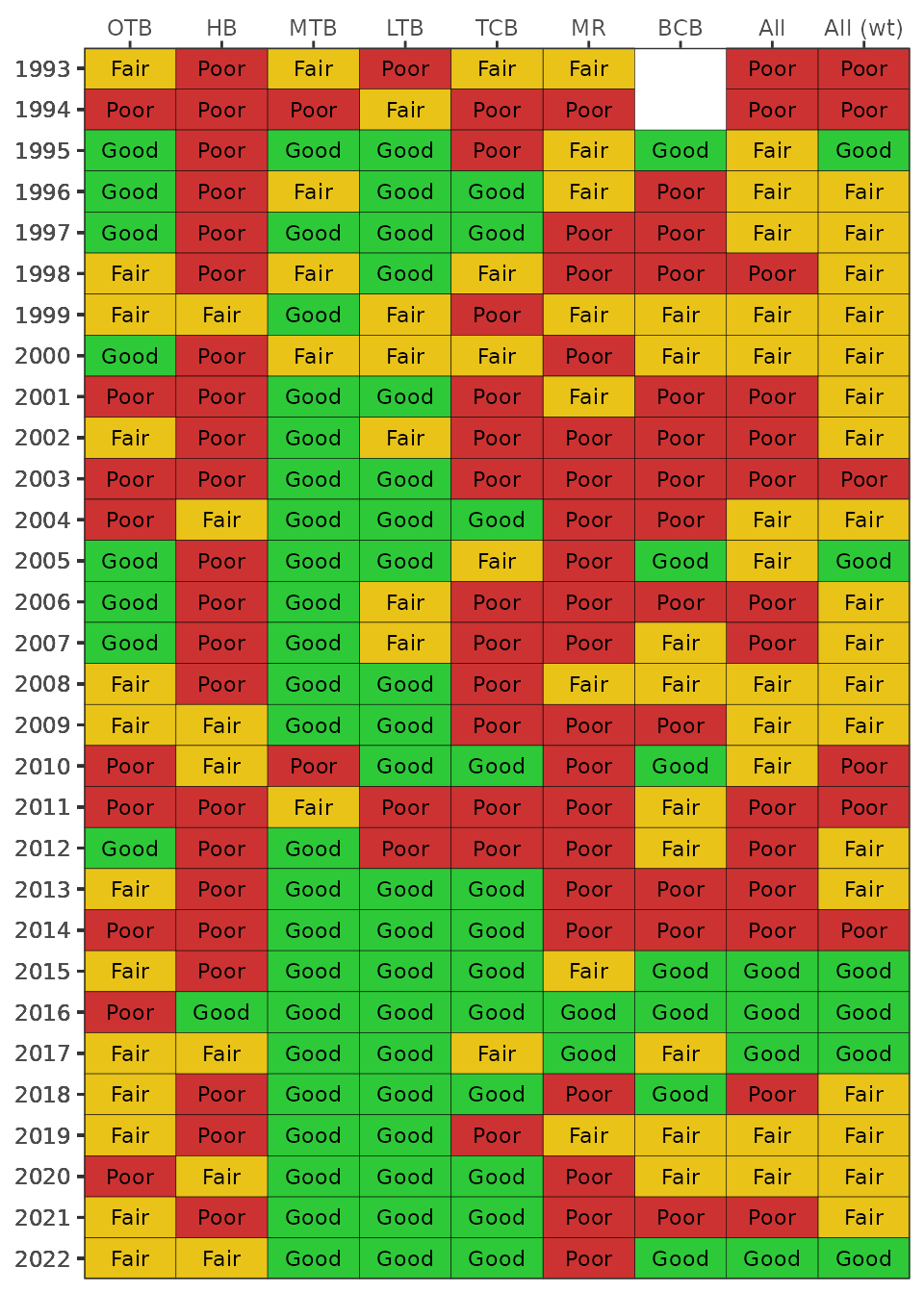
The matrix can also be produced as a plotly interactive plot by setting
plotly = TRUE inside the function.
show_tbbimatrix(tbbiscr, plotly = T)AZTI Marine Biotic Index (AMBI)
Background
The AZTI Marine Biotic Index (AMBI) is a measure of benthic community health based on the pollution sensitivity of the organisms found at a sampling station. Benthic macroinvertebrates are assigned to one of five ecological groups ranging from Group I (most sensitive, typical of clean conditions) to Group V (most tolerant, typical of heavily disturbed conditions) based on established taxonomic lists [3]. A Biotic Coefficient (BC) is then calculated as a weighted sum of the proportion of taxa records in each group:
Lower BC values indicate undisturbed conditions dominated by sensitive species, while higher values (approaching 7) indicate heavily stressed communities. Azoic stations (empty samples with no organisms) receive a BC of 7. An adjusted score on a 0 to 10 scale is also computed as , where higher values indicate healthier conditions.
Pollution categories are assigned based on the adjusted score: Unpolluted (above 8.29), Slightly Polluted (5.29 to 8.29), Meanly Polluted (2.89 to 5.29), Heavily Polluted (1.39 to 2.89), and Extremely Polluted (below 1.39). Azoic stations are assigned an adjusted score of zero and treated as Extremely Polluted.
The tbeptools package supports two AMBI variants calculated from the
same benthicdata object used for the TBBI. The standard
variant uses Gulf of Mexico ecological group assignments from [3], while the Tampa Bay-specific variant
(AMBI-TB) uses group assignments tailored to the local benthic community
[1]. Both variants use the same scoring
formula, where only the taxon-to-group mapping differs.
Calculating AMBI scores
AMBI scores by site are calculated using anlz_ambiscr().
The type argument selects the variant, defaulting to the
standard GOM assignments.
ambiscr <- anlz_ambiscr(benthicdata)
ambiscr
#> # A tibble: 4,915 × 23
#>    StationID StationNumber AreaAbbr FundingProject ProgramID ProgramName
#>        <int> <chr>         <chr>    <chr>              <int> <chr>
#>  1       448 02BBs301      MTB      Apollo Beach           4 Benthic Monitoring
#>  2       449 02BBs305      MTB      Apollo Beach           4 Benthic Monitoring
#>  3       450 02BBs307      MTB      Apollo Beach           4 Benthic Monitoring
#>  4       451 02BBs364      MTB      Apollo Beach           4 Benthic Monitoring
#>  5       452 02BBs369      MTB      Apollo Beach           4 Benthic Monitoring
#>  6       453 02BBs395      MTB      Apollo Beach           4 Benthic Monitoring
#>  7       454 02BBs397      MTB      Apollo Beach           4 Benthic Monitoring
#>  8       455 02BBs398      MTB      Apollo Beach           4 Benthic Monitoring
#>  9       456 02BBs401      MTB      Apollo Beach           4 Benthic Monitoring
#> 10       457 02BBs402      MTB      Apollo Beach           4 Benthic Monitoring
#> # ℹ 4,905 more rows
#> # ℹ 17 more variables: Latitude <dbl>, Longitude <dbl>, date <date>, yr <dbl>,
#> #   TotalGroupCount <int>, PercentG1 <dbl>, PercentG2 <dbl>, PercentG3 <dbl>,
#> #   PercentG4 <dbl>, PercentG5 <dbl>, BC <dbl>, AMBI <dbl>,
#> #   SitePollutionClassification <chr>, BioticIndex <chr>,
#> #   DominatingEcologicalGroup <chr>, BenthicCommunityHealth <chr>,
#> #   AMBICat <chr>
The Tampa Bay-specific variant is selected with
type = 'AMBI-TB'.
ambiscr_tb <- anlz_ambiscr(benthicdata, type = 'AMBI-TB')
ambiscr_tb
#> # A tibble: 4,915 × 23
#>    StationID StationNumber AreaAbbr FundingProject ProgramID ProgramName
#>        <int> <chr>         <chr>    <chr>              <int> <chr>
#>  1       448 02BBs301      MTB      Apollo Beach           4 Benthic Monitoring
#>  2       449 02BBs305      MTB      Apollo Beach           4 Benthic Monitoring
#>  3       450 02BBs307      MTB      Apollo Beach           4 Benthic Monitoring
#>  4       451 02BBs364      MTB      Apollo Beach           4 Benthic Monitoring
#>  5       452 02BBs369      MTB      Apollo Beach           4 Benthic Monitoring
#>  6       453 02BBs395      MTB      Apollo Beach           4 Benthic Monitoring
#>  7       454 02BBs397      MTB      Apollo Beach           4 Benthic Monitoring
#>  8       455 02BBs398      MTB      Apollo Beach           4 Benthic Monitoring
#>  9       456 02BBs401      MTB      Apollo Beach           4 Benthic Monitoring
#> 10       457 02BBs402      MTB      Apollo Beach           4 Benthic Monitoring
#> # ℹ 4,905 more rows
#> # ℹ 17 more variables: Latitude <dbl>, Longitude <dbl>, date <date>, yr <dbl>,
#> #   TotalGroupCount <int>, PercentG1 <dbl>, PercentG2 <dbl>, PercentG3 <dbl>,
#> #   PercentG4 <dbl>, PercentG5 <dbl>, BC <dbl>, TBAMBI <dbl>,
#> #   SitePollutionClassification <chr>, BioticIndex <chr>,
#> #   DominatingEcologicalGroup <chr>, BenthicCommunityHealth <chr>,
#> #   TBAMBICat <chr>
Both outputs include the Biotic Coefficient (BC), the
adjusted AMBI score (AMBI or TBAMBI), the
pollution category (AMBICat or TBAMBICat), and
ancillary descriptors (SitePollutionClassification,
BioticIndex, DominatingEcologicalGroup,
BenthicCommunityHealth).
Plotting results
The dominant AMBI pollution category for each bay segment and year
can be viewed as a matrix using show_ambimatrix().
Internally, the function summarizes the percent of sites in each
category per bay segment and year using anlz_ambimed(),
then identifies the plurality category for display. By default, a
rolling five-year window is applied from 2005 onward to smooth
inter-annual variability from reduced sampling effort in recent years,
similar to the TBBI.
show_ambimatrix(ambiscr_tb)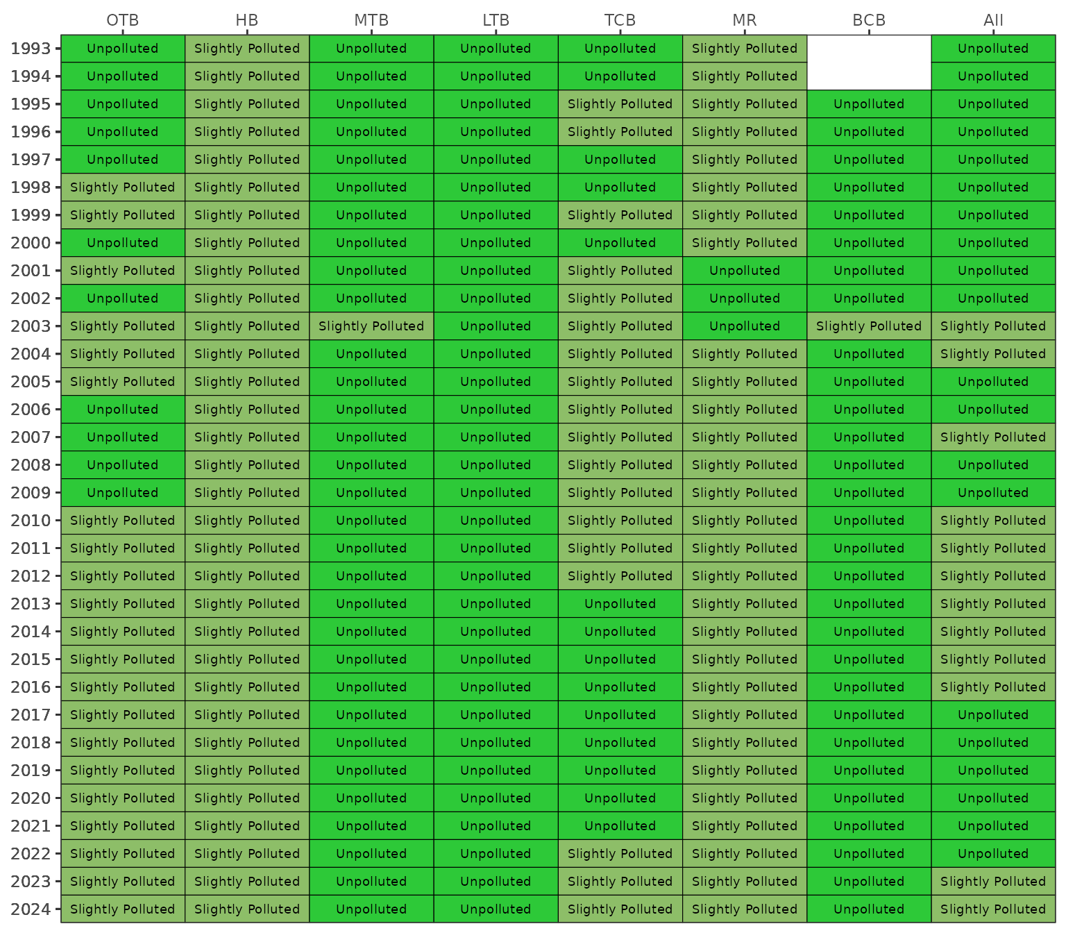
The matrix can also be produced as a plotly interactive plot.
show_ambimatrix(ambiscr_tb, plotly = TRUE)Mean annual adjusted AMBI scores can be plotted over time using
show_ambitrend(). The background shading identifies the
pollution category zones. Both AMBI variants can be overlaid on the same
plot by providing both scoring objects.
show_ambitrend(ambiscr, ambiscr_tb)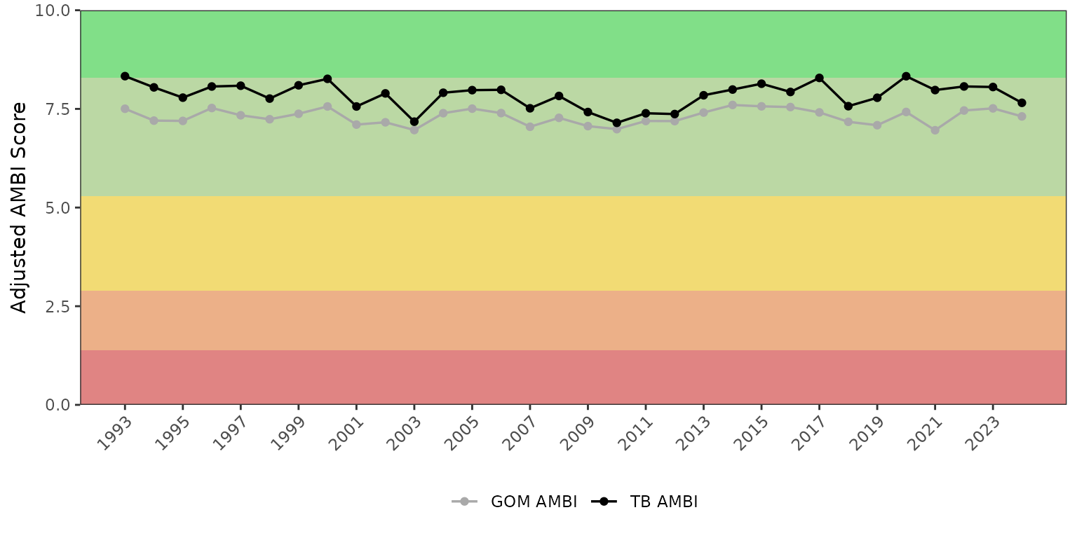
The same plot can be produced as an interactive plotly object.
show_ambitrend(ambiscr, ambiscr_tb, plotly = TRUE)By default, show_ambitrend() plots the mean adjusted
AMBI scores for all bay segments combined. The bay_segment
argument can be used to plot individual segments (or combinations)
instead.
show_ambitrend(ambiscr, ambiscr_tb, bay_segment = 'HB')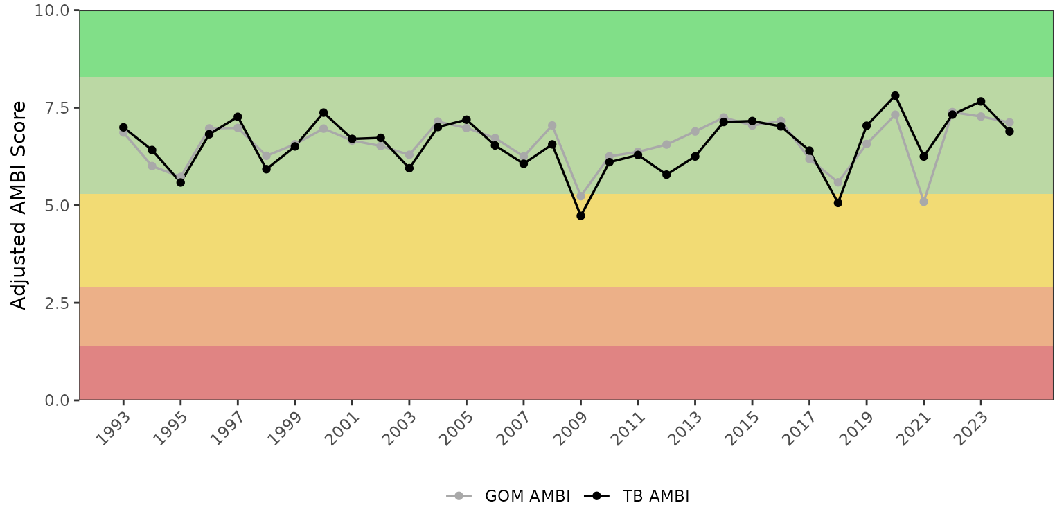
A summary table of the percent of sites in each AMBI category by bay
segment over a selected year range can be produced with
show_ambitab(). By default, the summaries are calculated
for all bay segments.
show_ambitab(ambiscr)Segment |
n |
Extremely Polluted |
Heavily Polluted |
Meanly Polluted |
Slightly Polluted |
Unpolluted |
|---|---|---|---|---|---|---|
OTB |
318 |
1.3% |
0.0% |
1.3% |
85.2% |
12.3% |
HB |
470 |
4.0% |
0.2% |
6.4% |
88.7% |
0.6% |
MTB |
332 |
0.3% |
0.0% |
0.0% |
84.6% |
15.1% |
LTB |
258 |
0.0% |
0.0% |
0.0% |
85.3% |
14.7% |
TCB |
129 |
0.0% |
0.8% |
1.6% |
90.7% |
7.0% |
MR |
237 |
0.0% |
0.0% |
1.3% |
97.0% |
1.7% |
BCB |
365 |
1.6% |
0.5% |
1.9% |
91.5% |
4.4% |
All |
2,109 |
1.4% |
0.2% |
2.2% |
88.7% |
7.5% |
Summarizing for individual bay segments or a different annual range
is also possible by specifying the bay_segment and
yrrng arguments, respectively.
show_ambitab(ambiscr, bay_segment = c('OTB', 'HB'), yrrng = c(2010, 2020))Segment |
n |
Extremely Polluted |
Heavily Polluted |
Meanly Polluted |
Slightly Polluted |
Unpolluted |
|---|---|---|---|---|---|---|
OTB |
91 |
3.3% |
0.0% |
0.0% |
89.0% |
7.7% |
HB |
99 |
3.0% |
0.0% |
8.1% |
86.9% |
2.0% |
All |
190 |
3.2% |
0.0% |
4.2% |
87.9% |
4.7% |
Additional sediment data
In addition to biological data, sediment contaminant concentrations are measured at sites within Tampa Bay. These include over 100 different constituents grouped broadly as metals, organics, physical, or other. The concentrations of these constituents can be compared relative to Threshold Effects Levels (TEL) or Potential Effects Levels (PEL), when available, as relative indications of the likelihood that the concentrations will have toxic effects on invertebrates that inhabit the sediments. The functions in tbeptools can be used to retrieve the sediment data and provide an indication of the concentrations relative to the TEL or PEL thresholds.
The read_importsediment() function will retrieve all
sediment data for Tampa Bay collected annually by the Environmental
Protection Commission of Hillsborough County. The data are retrieved
from the same
location as the biological data used to calculate the TBBI.
path <- '~/Desktop/sediment.zip'
sedimentdata <- read_importsediment(path, download_latest = T)
After the data are imported, you can view them from the assigned object.
sedimentdata
#> # A tibble: 231,727 × 24
#>    ProgramId ProgramName   FundingProject    yr AreaAbbr StationID StationNumber
#>        <int> <chr>         <chr>          <int> <chr>        <int> <chr>
#>  1         4 Benthic Moni… TBEP            1993 HB            2463 93HB15
#>  2         4 Benthic Moni… TBEP            1993 HB            2463 93HB15
#>  3         4 Benthic Moni… TBEP            1993 HB            2463 93HB15
#>  4         4 Benthic Moni… TBEP            1993 HB            2463 93HB15
#>  5         4 Benthic Moni… TBEP            1993 HB            2463 93HB15
#>  6         4 Benthic Moni… TBEP            1993 HB            2463 93HB15
#>  7         4 Benthic Moni… TBEP            1993 HB            2463 93HB15
#>  8         4 Benthic Moni… TBEP            1993 HB            2463 93HB15
#>  9         4 Benthic Moni… TBEP            1993 HB            2463 93HB15
#> 10         4 Benthic Moni… TBEP            1993 HB            2463 93HB15
#> # ℹ 231,717 more rows
#> # ℹ 17 more variables: Latitude <dbl>, Longitude <dbl>, Replicate <chr>,
#> #   SedResultsType <chr>, Parameter <chr>, ValueAdjusted <dbl>, Units <chr>,
#> #   Qualifier <chr>, MDLnum <chr>, PQLnum <chr>, TEL <dbl>, PEL <dbl>,
#> #   BetweenTELPEL <chr>, ExceedsPEL <chr>, PELRatio <dbl>,
#> #   PreparationDate <chr>, AnalysisTimeMerge <chr>
The show_sedimentmap() function can be used to create
maps of selected parameters relative to TEL and PEL values. Green points
show concentrations below the TEL, yellow points show concentrations
between the TEL and PEL, and red points show concentrations above the
PEL. The applicable TEL and PEL values for the parameter are indicated
in the legend. The selected stations are those that are sampled in the
years within the yrrng argument.
show_sedimentmap(sedimentdata, param = 'Arsenic', yrrng = c(1993, 2024))A single year of data can be shown as well.
show_sedimentmap(sedimentdata, param = 'Arsenic', yrrng = 2024)A map showing only the concentrations is returned if TEL and PEL values are not available for a parameter.
show_sedimentmap(sedimentdata, param = 'Selenium', yrrng = c(1993, 2024))Maps for total contaminant values (e.g., Total DDT, Total PAH, Total
PCB, Total LMW PAH, Total HMW PAH) can also be returned. Although the
totals are not included in the sedimentdata object, they
are calculated by tbeptools using the anlz_sedimentaddtot()
function. Simply entering the name of the total parameter in the
show_sedimentmap() function will produce the summary
map.
show_sedimentmap(sedimentdata, param = 'Total DDT', yrrng = c(1993, 2024))The PEL ratio can also be used to assess relative sediment quality
given the measured contaminants. The show_sedimentpelmap()
function creates a map of average PEL ratios graded from A to F for
benthic stations monitored in Tampa Bay. The PEL ratio is the
contaminant concentration divided by the Potential Effects Levels (PEL)
that applies to a contaminant, if available. Higher ratios and lower
grades indicate sediment conditions that are likely unfavorable for
invertebrates. The station average combines the PEL ratios across all
contaminants measured at a station.
show_sedimentpelmap(sedimentdata, yrrng = c(1993, 2024))The average PEL ratios and grades used to create the map can also be
returned as a data frame using anlz_sedimentpel().
anlz_sedimentpel(sedimentdata, yrrng = c(1993, 2024))
#> # A tibble: 2,321 × 7
#>       yr AreaAbbr StationNumber Latitude Longitude PELRatio Grade
#>    <int> <chr>    <chr>            <dbl>     <dbl>    <dbl> <fct>
#>  1  1993 HB       93HB15            27.8     -82.4  0.0157  B
#>  2  1993 HB       93HB16            27.8     -82.5  0.0261  C
#>  3  1993 HB       93HB23            27.9     -82.4  0.0174  B
#>  4  1993 LTB      93LTB24           27.7     -82.6  0.0124  B
#>  5  1993 LTB      93LTB25           27.6     -82.6  0.0189  B
#>  6  1993 LTB      93LTB26           27.6     -82.7  0.00997 B
#>  7  1993 LTB      93LTB27           27.6     -82.7  0.0125  B
#>  8  1993 LTB      93LTB28           27.6     -82.7  0.0887  D
#>  9  1993 LTB      93LTB29           27.6     -82.6  0.0350  C
#> 10  1993 LTB      93LTB30           27.6     -82.6  0.0496  C
#> # ℹ 2,311 more rows
Plots of bay segment averages of sediment concentrations for selected
parameters can be created with show_sedimentave(). The plot
includes appropriate lines for the TEL and PEL values, as well the grand
mean across all segments. The former are omitted from the plot if
unavailable for a selected parameter.
show_sedimentave(sedimentdata, param = 'Arsenic', yrrng = c(1993, 2024))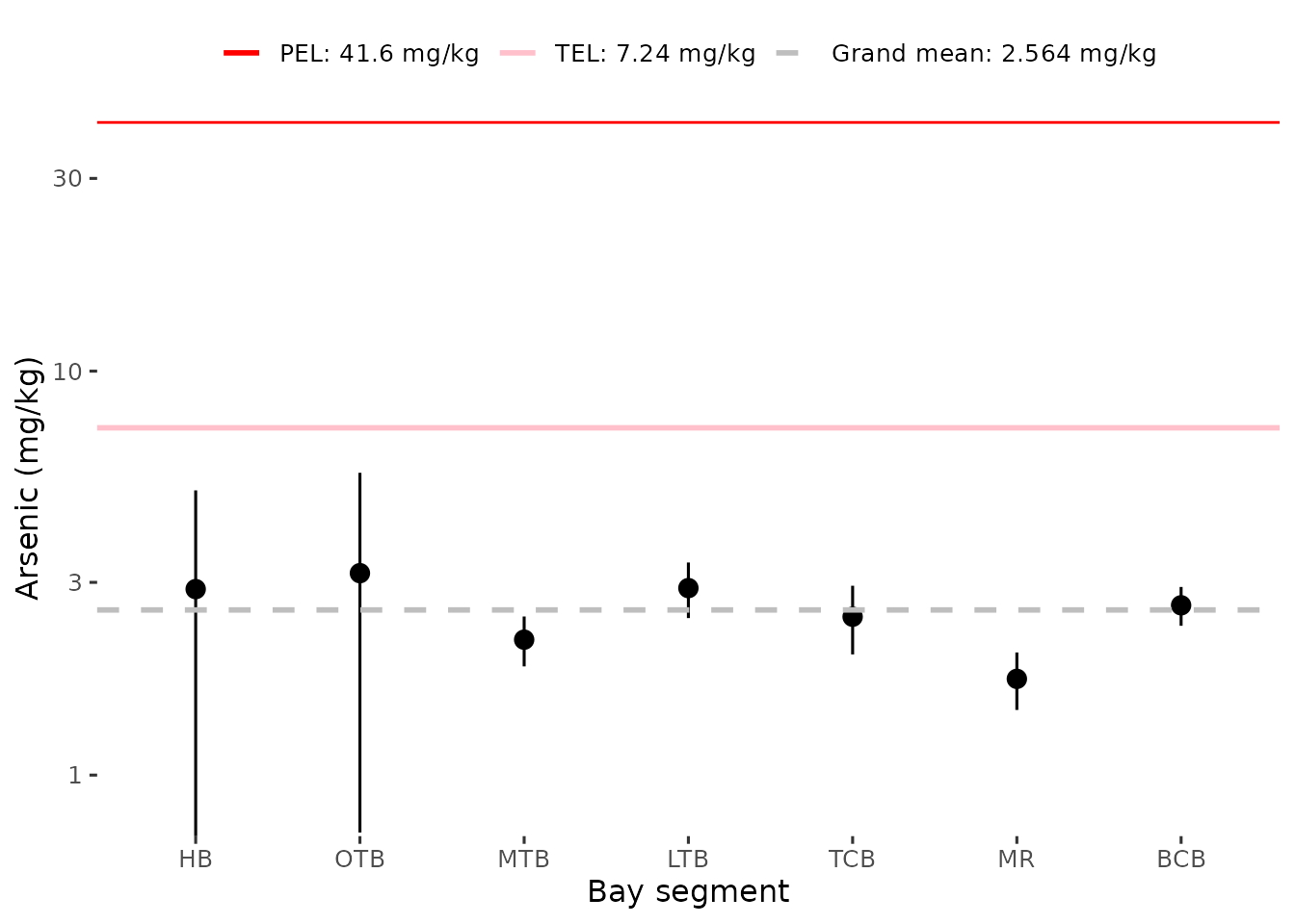
The same plot can be returned as an interactive plotly object using
plotly = T.
show_sedimentave(sedimentdata, param = 'Arsenic', yrrng = c(1993, 2024), plotly = T)The values used in the plot can be returned with
anlz_sedimentave().
anlz_sedimentave(sedimentdata, param = 'Arsenic', yrrng = c(1993, 2024))
#> # A tibble: 7 × 8
#>   AreaAbbr   TEL   PEL Units   ave   lov   hiv grandave
#>   <fct>    <dbl> <dbl> <chr> <dbl> <dbl> <dbl>    <dbl>
#> 1 BCB       7.24  41.6 mg/kg  2.63 2.34   2.92     2.56
#> 2 HB        7.24  41.6 mg/kg  2.89 0.706  5.07     2.56
#> 3 LTB       7.24  41.6 mg/kg  2.90 2.45   3.36     2.56
#> 4 MR        7.24  41.6 mg/kg  1.73 1.45   2.01     2.56
#> 5 MTB       7.24  41.6 mg/kg  2.16 1.86   2.47     2.56
#> 6 OTB       7.24  41.6 mg/kg  3.16 0.721  5.60     2.56
#> 7 TCB       7.24  41.6 mg/kg  2.47 1.99   2.94     2.56
As before, the total contaminant values (e.g., Total DDT, Total PAH,
Total PCB, Total LMW PAH, Total HMW PAH) can also be returned even
though they are not included in the sedimentdata object.
The anlz_sedimentaddtot() function is used to calculate the
totals within anlz_sedimentave().
anlz_sedimentave(sedimentdata, param = 'Total DDT', yrrng = c(1993, 2024))
#> # A tibble: 7 × 8
#>   AreaAbbr   TEL   PEL Units   ave   lov   hiv grandave
#>   <fct>    <dbl> <dbl> <chr> <dbl> <dbl> <dbl>    <dbl>
#> 1 BCB       3.89  51.7 ug/kg 0.547 0.371 0.724    0.676
#> 2 HB        3.89  51.7 ug/kg 1.71  0.845 2.58     0.676
#> 3 LTB       3.89  51.7 ug/kg 0.214 0.104 0.325    0.676
#> 4 MR        3.89  51.7 ug/kg 0.799 0.502 1.10     0.676
#> 5 MTB       3.89  51.7 ug/kg 0.424 0.280 0.569    0.676
#> 6 OTB       3.89  51.7 ug/kg 0.475 0.267 0.682    0.676
#> 7 TCB       3.89  51.7 ug/kg 0.565 0.196 0.934    0.676
A similar plot of the bay segment averages for the average PEL ratios
can be created with show_sedimentpelave(). The colors
indicate the grades for A (green) to F (red).
show_sedimentpelave(sedimentdata, yrrng = c(1993, 2024))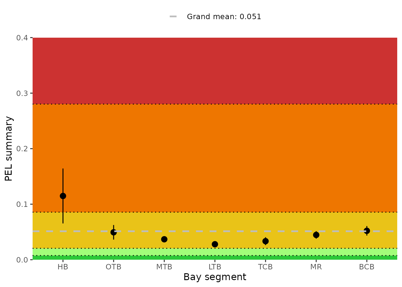
The same plot can be returned as an interactive plotly object using
plotly = T.
show_sedimentpelave(sedimentdata, yrrng = c(1993, 2024), plotly = T)The values used in the plot can be returned with
anlz_sedimentpelave().
anlz_sedimentpelave(sedimentdata, yrrng = c(1993, 2024))
#> # A tibble: 7 × 5
#>   AreaAbbr    ave    lov    hiv grandave
#>   <fct>     <dbl>  <dbl>  <dbl>    <dbl>
#> 1 BCB      0.0521 0.0435 0.0606   0.0513
#> 2 HB       0.115  0.0654 0.164    0.0513
#> 3 LTB      0.0279 0.0246 0.0312   0.0513
#> 4 MR       0.0447 0.0380 0.0514   0.0513
#> 5 MTB      0.0368 0.0322 0.0414   0.0513
#> 6 OTB      0.0494 0.0363 0.0625   0.0513
#> 7 TCB      0.0334 0.0264 0.0404   0.0513
The show_sedimentalratio() function creates a plot of a
selected metal parameter against Aluminum. This plot provides
information on the concentration of the parameter relative to background
levels, where Aluminum is present as a common metal in the Earth’s
crust. An elevated ratio of a metal parameter relative to aluminum
suggests it is higher than background concentrations [4]. The linear fit of a log-log model is shown
as a solid black line, with 95% prediction intervals. The TEL/PEL
values, if available, are also shown as horizontal red lines.
show_sedimentalratio(sedimentdata, param = 'Zinc', bay_segment = c('HB', 'LTB'))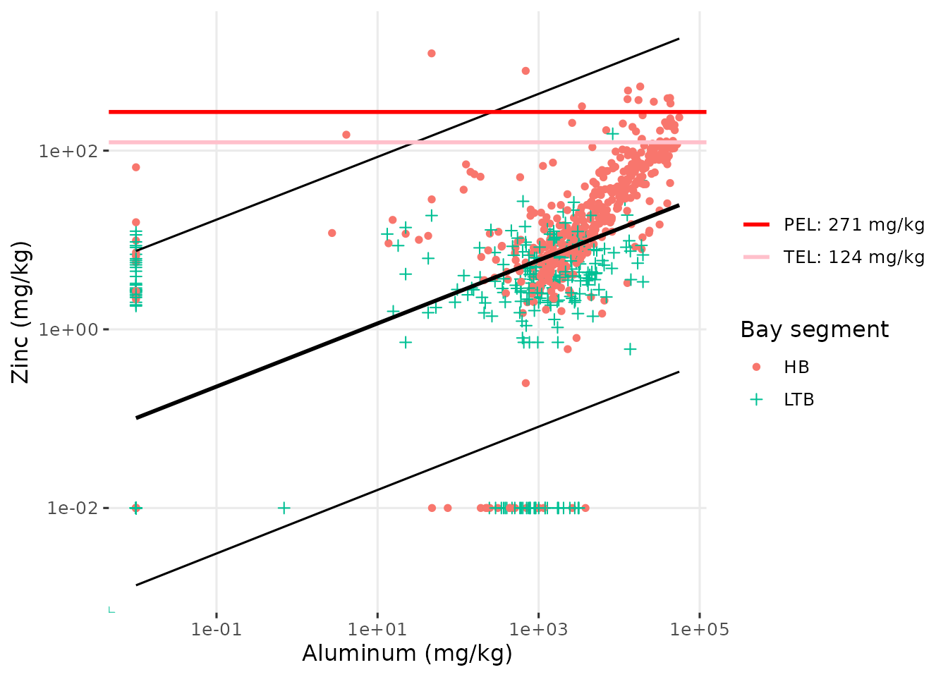
The same plot can be returned as an interactive plotly object using
plotly = T.
show_sedimentalratio(sedimentdata, param = 'Zinc', bay_segment = c('HB', 'LTB'), plotly = T)