Introduction
Introduction.RmdBasic use
First we load the peptools package. Note that we do not need to install it every time we use R, but we do need to load the package.
library(peptools)The package includes a pepstations data object that
includes metadata for each station, including lat/lon and bay segment.
We can use the sf and dplyr package to make this a spatial data object,
then plot it with mapview (you may need to install these packages if you
don’t have them). Note that the peptools package has built-in mapping
functions, this example just shows how to create a map from scratch.
library(sf)
library(dplyr)
library(mapview)

locs <- pepstations %>%
  sf::st_as_sf(coords = c('Longitude', 'Latitude'), crs = 4326) %>%
  dplyr::mutate(bay_segment = as.character(bay_segment))

mapview(locs, zcol = 'bay_segment', layer.name = 'Bay segment')
The pepseg data object also included with the package
shows the polygons for the bay segments.
mapview(pepseg)The water quality data can be imported using the
read_pepwq() function. A compressed folder that includes
the data can be downloaded from here.
After the data are downloaded and extracted, the Excel file with the raw
data is named “Peconics SCDHS WQ data - 1976 - 2021.xlsx”, or something
similar depending on when the data were downloaded. The location of this
file on your computer is passed to the import function. Below, a local
file renamed as “currentdata.xlsx” that contains the water quality data
is imported.
dat <- read_pepwq('../inst/extdata/currentdata.xlsx')
head(dat)
#> # A tibble: 6 × 11
#>   Date       BayStation name  value status    yr    mo StationName   bay_segment
#>   <date>     <chr>      <chr> <dbl> <chr>  <dbl> <dbl> <chr>         <fct>
#> 1 1990-01-31 60113      chla    4.8 ""      1990     1 Little Pecon… 2
#> 2 1990-01-31 60113      sd      8   ""      1990     1 Little Pecon… 2
#> 3 1990-01-31 60114      chla    2.8 ""      1990     1 Paradise Poi… 2
#> 4 1990-01-31 60114      sd     12   ""      1990     1 Paradise Poi… 2
#> 5 1990-01-31 60115      chla    8.5 ""      1990     1 Orient Harbor 3
#> 6 1990-01-31 60115      sd      7   ""      1990     1 Orient Harbor 3
#> # ℹ 2 more variables: Longitude <dbl>, Latitude <dbl>
The raw data includes multiple fields, but only the chlorophyll,
secchi, and total nitrogen data are retained for reporting. The data are
in long format with the name column showing which
observation (chlorophyll, secchi, or total nitrogen) the row
value shows and the status showing if the
observation was above or below detection (indicated as >
or <, secchi only). Each station is also grouped by
major bay segment, defined as 1a, 1b, 2, 3.
A quick view of the number of observations and length of record at each station shows that effort was not continuous.
library(ggplot2)

toplo <- dat %>%
  select(bay_segment, BayStation, yr, name, value) %>%
  group_by(bay_segment, BayStation, yr, name) %>%
  summarise(`Obs. (n)` = n())

p <- ggplot(toplo, aes(x = yr, y = BayStation, fill = `Obs. (n)`)) +
  geom_tile()+ #colour = 'lightgrey') +
  facet_grid(bay_segment ~ name, scales = 'free_y', space = 'free_y') +
  theme_bw() +
  theme(
    panel.grid.major = element_blank(),
    panel.grid.minor= element_blank(),
    strip.background = element_blank(),
    axis.title.x = element_blank(),
    legend.position = 'top',
    axis.text.y = element_text(size = 7)
  ) +
  scale_fill_viridis_c()

p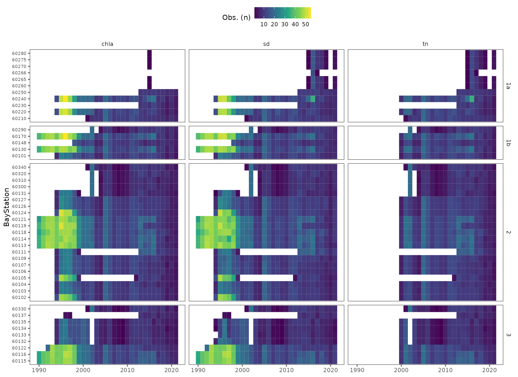
The function anlz_pepdat() summarizes the station data
by bay segment. The function returns annual medians and monthly medians
by year for chlorophyll, secchi depth, and total nitrogen. The
chlorophyll and secchi summaries are then used to determine if bay
segment targets for water quality are met using the
anlz_attain() and anlz_attainpep()
functions.
Below shows how to use anlz_pepdat() to summarize the
data by bay segment to estimate annual and monthly medians for
chlorophyll, secchi depth, and total nitrogen. The output is a
two-element list for the annual (ann) and monthly (mos) medians by
segment.
medpep <- anlz_medpep(dat)
medpep
#> $ann
#> # A tibble: 1,260 × 5
#>    bay_segment    yr   val est    var
#>    <fct>       <dbl> <dbl> <chr>  <chr>
#>  1 1a           2024  6.29 lwr.ci chla
#>  2 1a           2024  8.39 medv   chla
#>  3 1a           2024 11.9  upr.ci chla
#>  4 1a           2023  6.6  lwr.ci chla
#>  5 1a           2023  8.53 medv   chla
#>  6 1a           2023 10.8  upr.ci chla
#>  7 1a           2022  4.16 lwr.ci chla
#>  8 1a           2022  7.53 medv   chla
#>  9 1a           2022  9.97 upr.ci chla
#> 10 1a           2021  8.4  lwr.ci chla
#> # ℹ 1,250 more rows
#>
#> $mos
#> # A tibble: 5,040 × 6
#>    bay_segment    yr    mo   val est   var
#>    <fct>       <dbl> <dbl> <dbl> <chr> <chr>
#>  1 1a           2024    12  8.82 medv  chla
#>  2 1a           2024    11 30.5  medv  chla
#>  3 1a           2024    10 15.0  medv  chla
#>  4 1a           2024     9 24.5  medv  chla
#>  5 1a           2024     8 24.9  medv  chla
#>  6 1a           2024     7 11.8  medv  chla
#>  7 1a           2024     6 11.6  medv  chla
#>  8 1a           2024     5  4.79 medv  chla
#>  9 1a           2024     4  3.50 medv  chla
#> 10 1a           2024     3  2.24 medv  chla
#> # ℹ 5,030 more rows
This output can then be further analyzed with
anlz_attainpep() to determine if the bay segment outcomes
are met in each year for chlorophyll and secchi depth. The results are
used by the plotting functions described below. In short, the
chl_sd column indicates the categorical outcome for
chlorophyll and secchi for each segment. The outcomes are integer values
from zero to three. The relative exceedances of water quality thresholds
for each segment, both in duration and magnitude, are indicated by
higher integer values.
anlz_attainpep(medpep)
#> # A tibble: 140 × 4
#>    bay_segment    yr chla_sd outcome
#>    <fct>       <dbl> <chr>   <chr>
#>  1 1a           2024 3_3     red
#>  2 1a           2023 3_3     red
#>  3 1a           2022 2_2     red
#>  4 1a           2021 3_2     red
#>  5 1a           2020 2_NA    NA
#>  6 1a           2019 2_3     red
#>  7 1a           2018 2_3     red
#>  8 1a           2017 3_3     red
#>  9 1a           2016 3_3     red
#> 10 1a           2015 2_3     red
#> # ℹ 130 more rows
Plotting
The plotting functions are used to view station data, long-term trends for each bay segment, and annual results for the overall water quality assessment.
The show_sitemappep() function produces an interactive
map of medians of water quality conditions at each station. Medians can
be shown for chlorophyll, secchi depth, or total nitrogen and for all
stations or only stations from selected bay segments. Each point on the
map shows the median for the parameter, with the size and color of the
point in proportion to the other median values shown on the map. The
color scale for the median shows higher concentrations of
chlorophyll/total nitrogen or shallower secchi depths in red and lower
concentrations of chlorophyll/total nitrogen or deeper secchi depths in
blue. Hovering the mouse pointer over a site location will indicate the
site name and the median value. Clicking on a station point will reveal
the underlying plot data.
Here, the 2020 chlorophyll medians are shown for stations in all bay segments.
show_sitemappep(dat, yrsel = 2021)Medians for a given month can also be shown.
show_sitemappep(dat, mosel = 7)A different year, parameter, and bay segment can also be chosen. Note that the size and color ramps are reversed for secchi depth, such that smaller and bluer points indicate larger secchi values.
show_sitemappep(dat, yrsel = 2010, param = 'sd', bay_segment = c('2', '3'))By default, the color and size scaling in
show_sitemappep() is relative to only the points on the
map. You can view scaling relative to all values in the dataset (across
time and space) to get a sense of how the values for the selected year
compare to the rest of the record. This can be done by changing the
relative argument to TRUE.
show_sitemappep(dat, yrsel = 2021, relative = T)The scaling is also sensitive to outliers. The default is to use the
maximum scaling as the 99th percentile value observed in the entire
dataset for the chosen parameter. Otherwise, results that are visually
difficult to interpret will be returned if the absolute maximum value is
used to set the scale. If, however, you want to see scaling relative to
a smaller quantile, you can change the value with the
maxrel argument. The size and color ramps will be scaled to
the defined upper quantile value. The actual observed value at a point
will always be visible on mouseover.
show_sitemappep(dat, yrsel = 2021, relative = T, maxrel = 0.8)The show_thrpep() function provides a more descriptive
assessment of annual trends for a chosen bay segment relative to
thresholds. In this plot, we show the annual medians and non-parametric
confidence internals (95%) across stations for a segment. The red line
shows annual trends and the horizontal blue line indicates the threshold
for chlorophyll-a.
show_thrpep(dat, bay_segment = "1a", param = "chla")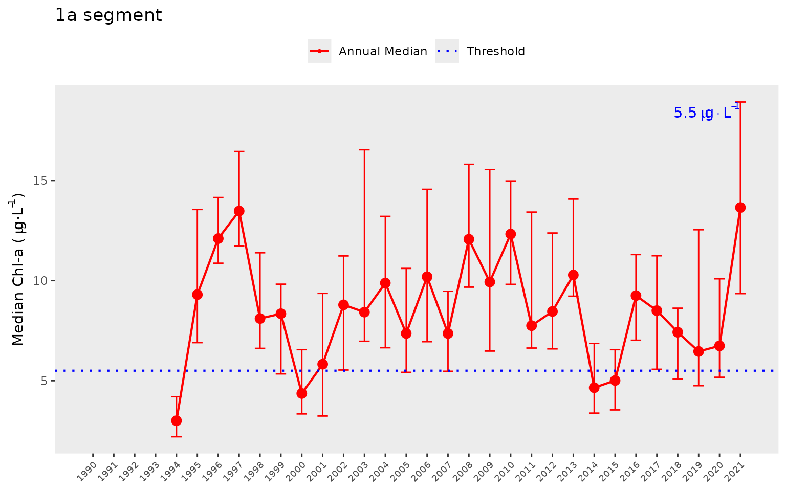
We can show the same plot but for secchi depth by changing the
param = "chla" to param = "sd". Note the
change in the horizontal reference lines for the secchi depth target.
Secchi trends must also be interpreted inversely to chlorophyll, such
that lower values generally indicate less desirable water quality.
show_thrpep(dat, bay_segment = "1a", param = "sd")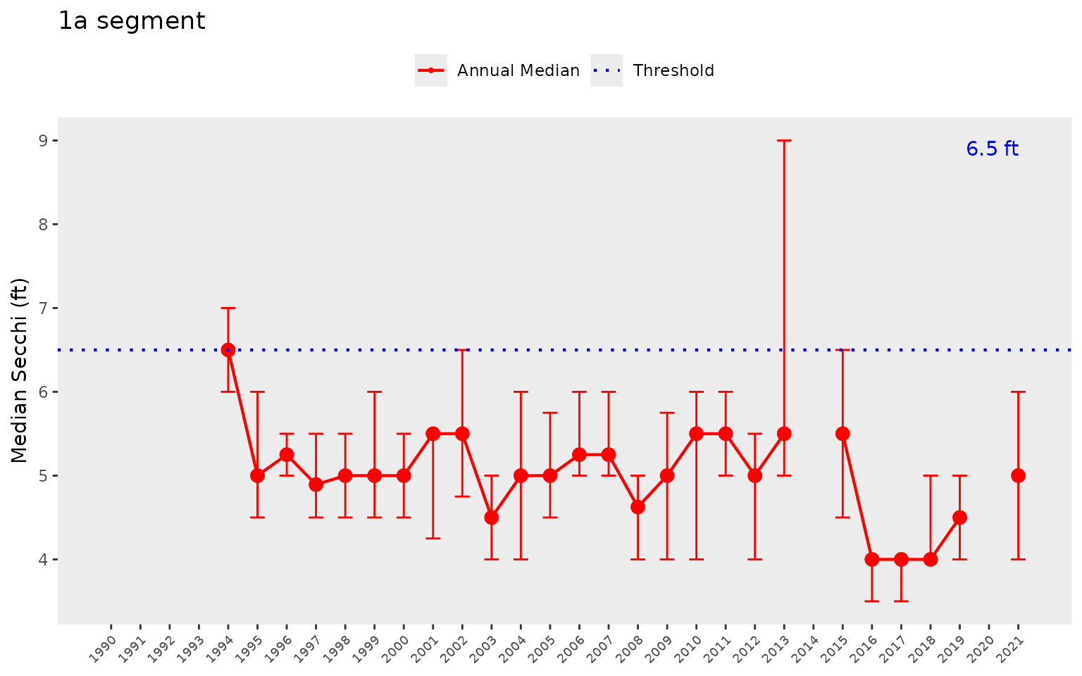
Total nitrogen can also be plotted.
show_thrpep(dat, bay_segment = "1a", param = "tn")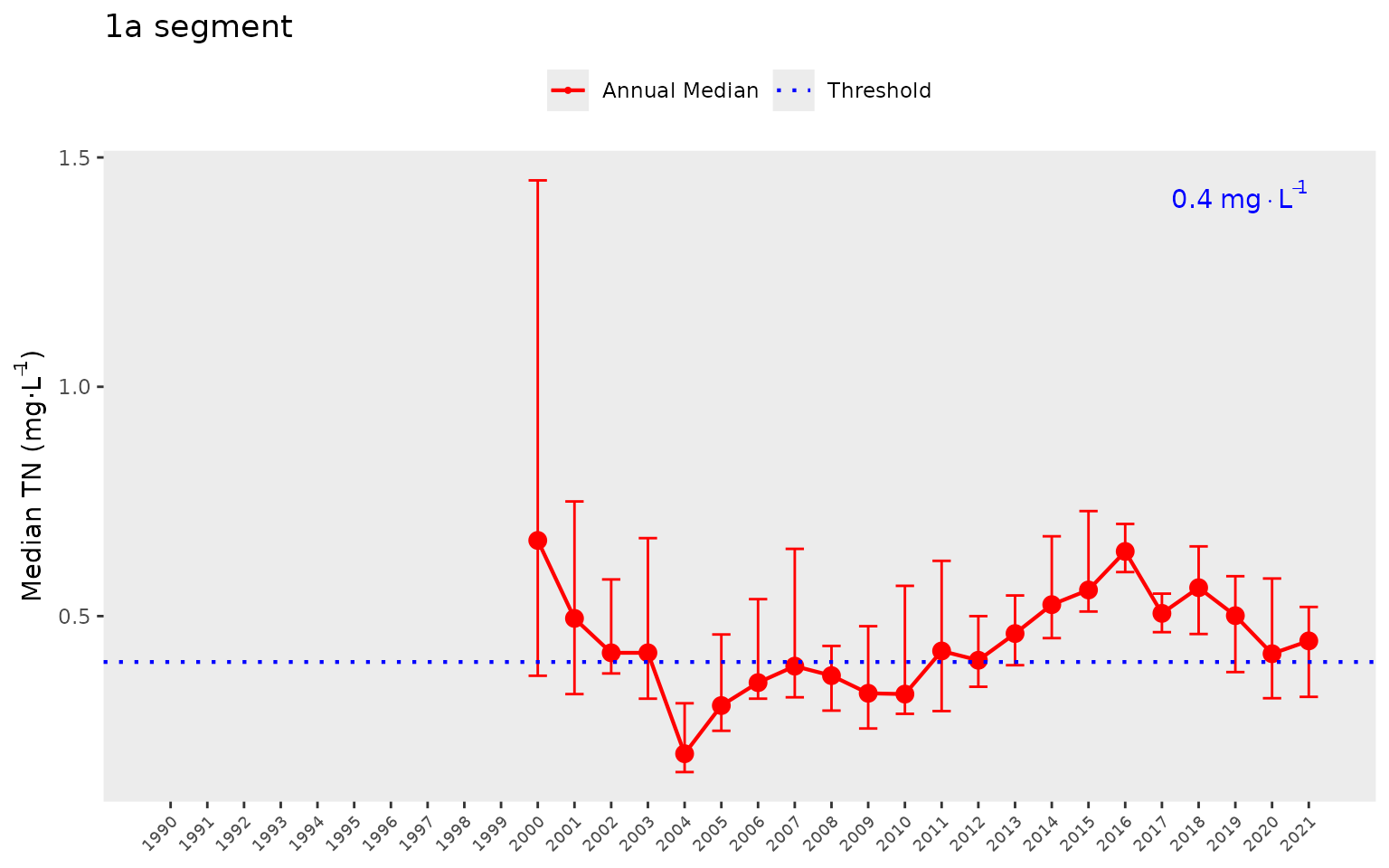
The year range to plot can also be specified using the
yrrng argument, where the default is
yrrng = c(1990, 2020).
show_thrpep(dat, bay_segment = "1a", param = "chla", yrrng = c(1976, 2021))
The show_allthrpep() function is a slight modification
of show_thrpep() that shows annual median results for all
bay segments combined. It accepts similar arguments as
show_thrpep(). Note that threshold values for chlorophyll-a
and Secchi depth can also be shown because the thresholds do not vary
between segments. A modification fo the function will be required if
these thresholds are modified for specific bay segments.
show_allthrpep(dat, param = "chla")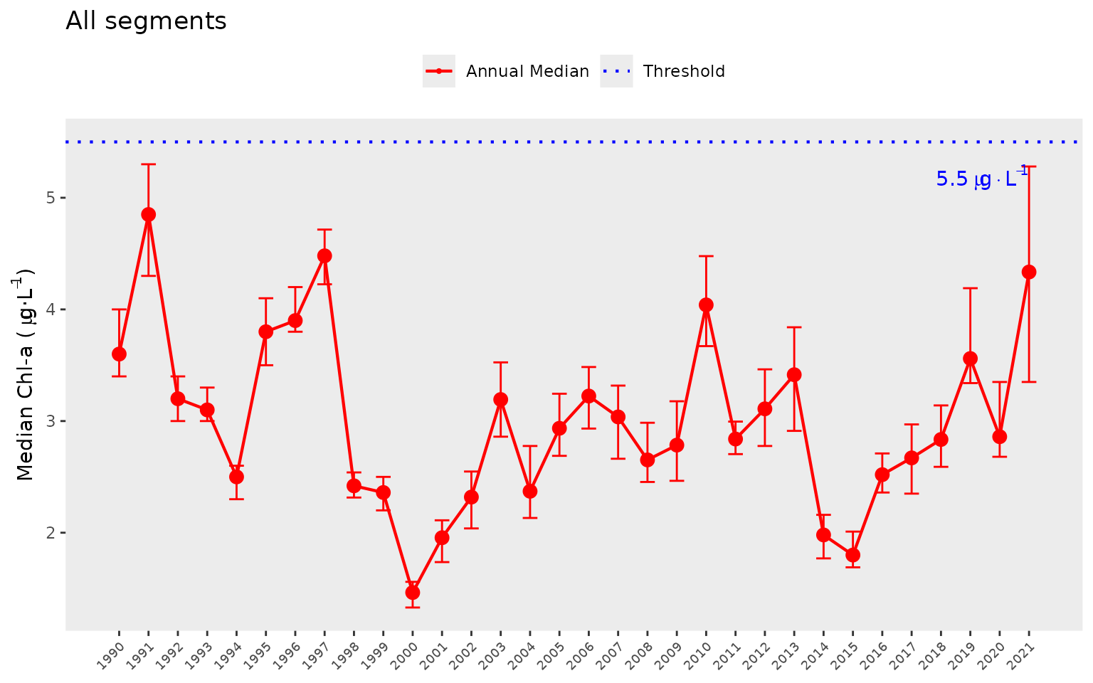
The show_thrpep() function uses results from the
anlz_medpep() function. For example, you can retrieve the
values from the above plot as follows:
dat %>%
  anlz_medpep %>%
  .[['ann']] %>%
  filter(bay_segment == '1a') %>%
  filter(var == 'chla') %>%
  filter(yr >= 1988 & yr <= 2021)
#> # A tibble: 96 × 5
#>    bay_segment    yr   val est    var
#>    <fct>       <dbl> <dbl> <chr>  <chr>
#>  1 1a           2021  8.4  lwr.ci chla
#>  2 1a           2021 10.3  medv   chla
#>  3 1a           2021 17    upr.ci chla
#>  4 1a           2020  5.17 lwr.ci chla
#>  5 1a           2020  6.74 medv   chla
#>  6 1a           2020 10.1  upr.ci chla
#>  7 1a           2019  4.75 lwr.ci chla
#>  8 1a           2019  6.46 medv   chla
#>  9 1a           2019 12.5  upr.ci chla
#> 10 1a           2018  5.08 lwr.ci chla
#> # ℹ 86 more rows
Similarly, the show_boxpep() function provides an
assessment of seasonal changes in chlorophyll, secchi depth, or total
nitrogen values by bay segment. The most recent year is highlighted in
red by default. This allows a simple evaluation of how the most recent
year compared to historical averages. The threshold value is shown in
blue text and as the dotted line (not shown for total nitrogen). This is
the same dotted line shown in show_thrpep().
show_boxpep(dat, param = 'chla', bay_segment = "1a")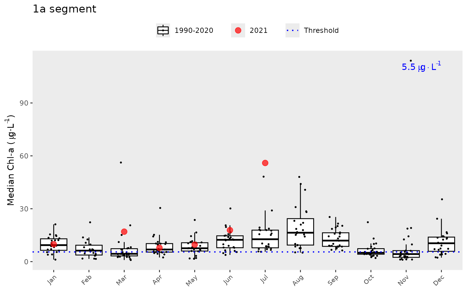
show_boxpep(dat, param = 'sd', bay_segment = "3")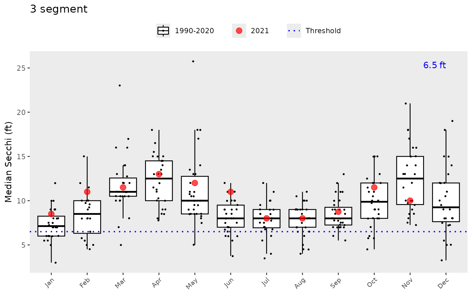
A different subset of years and selected year of interest can also be
viewed by changing the yrrng and yrsel
arguments. Here we show 1980 compared to monthly averages for the last
ten years.
show_boxpep(dat, param = 'chla', bay_segment = "1a", yrrng = c(2008, 2018), yrsel = 1990)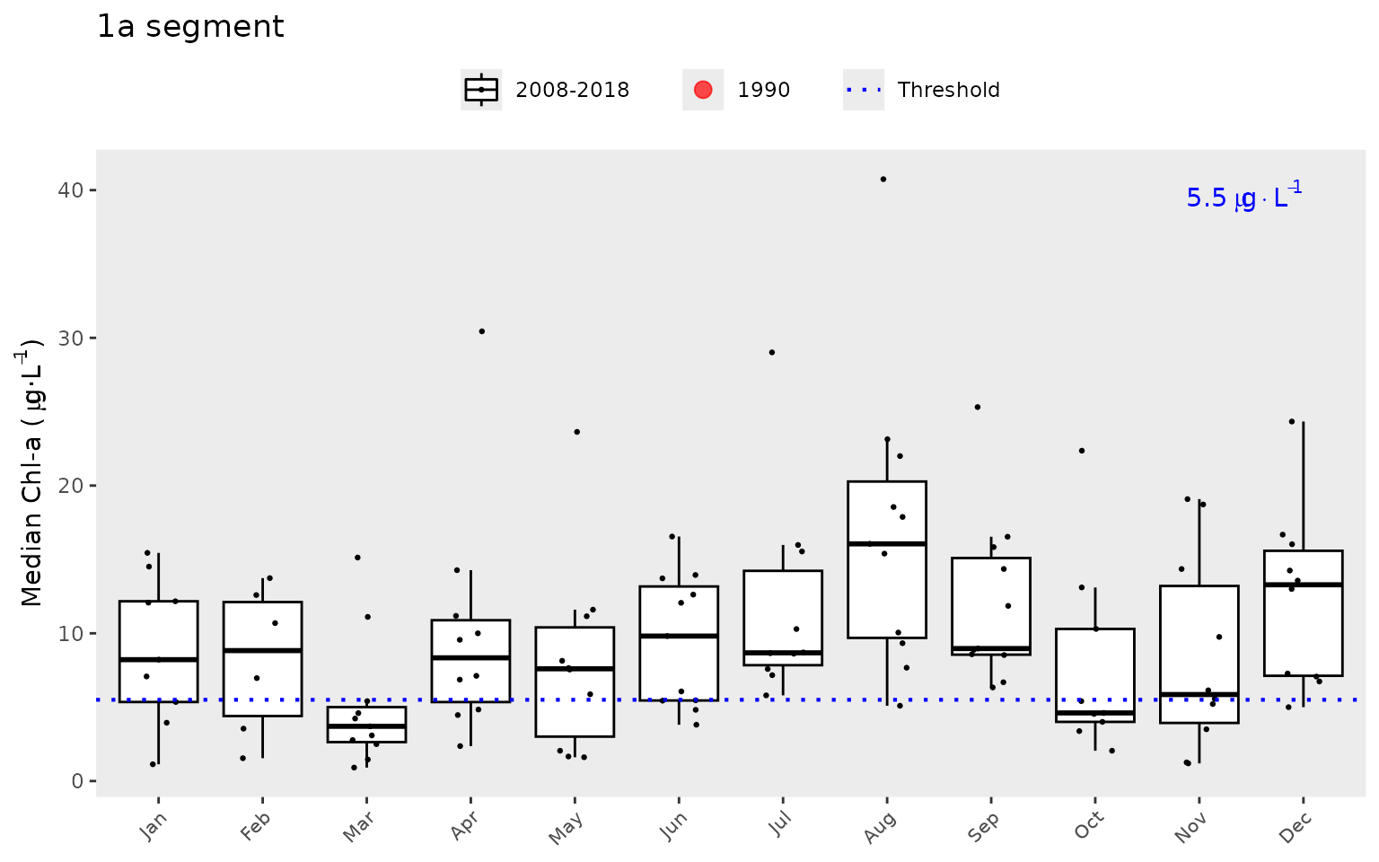
The show_thrpep() function is useful to understand
annual variation in chlorophyll, secchi, or total nitrogen in each bay
segment. For chlorophyll and secchi, the information from these plots
can provide an understanding of how the annual reporting outcomes are
determined. An outcome integer from zero to three is assigned to each
bay segment for each annual estimate of chlorophyll and secchi depth.
These outcomes are based on both the exceedance of the annual estimate
above the threshold (blue lines in show_thrpep()) and
duration of the exceedance for the years prior. The following graphic
describes this logic [1].
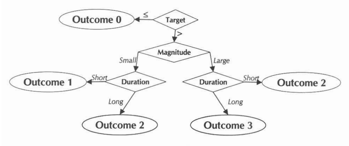
Outcomes for annual estimates of water quality are assigned an integer value from zero to three depending on both magnitude and duration of the exceedence.
For the Peconic Estuary, light attenuation is replaced with Secchi
depth. The outcomes above are assigned for both chlorophyll and secchi
depth. The duration criteria are determined based on whether the
exceedance was observed for years prior to the current year. The
exceedance criteria for chlorophyll and light-attenuation are currently
the same for each segment. The peptools package contains a
peptargets data file that is a reference for determining
annual outcomes. This file is loaded automatically with the package and
can be viewed from the command line.
peptargets
#> # A tibble: 4 × 5
#>   bay_segment name  sd_thresh chla_thresh tn_thresh
#>   <fct>       <fct>     <dbl>       <dbl>     <dbl>
#> 1 1a          1a          6.5         5.5       0.4
#> 2 1b          1b          6.5         5.5       0.4
#> 3 2           2           6.5         5.5       0.4
#> 4 3           3           6.5         5.5       0.4
The final plotting function is show_matrixpep(), which
creates an annual reporting matrix that reflects the combined outcomes
for chlorophyll and secchi depth. Tracking the attainment outcomes
provides the framework from which bay management actions can be
developed and initiated. For each year and segment, a color-coded
management action is assigned:
Stay the Course: Continue planned projects. Report data via annual progress reports and Baywide Environmental Monitoring Report.
Caution: Review monitoring data and nitrogen loading estimates. Begin/continue TAC and Management Board development of specific management recommendations.
On Alert: Finalize development and implement appropriate management actions to get back on track.
The management category or action is based on the combination of outcomes for chlorophyll and secchi depth [1].
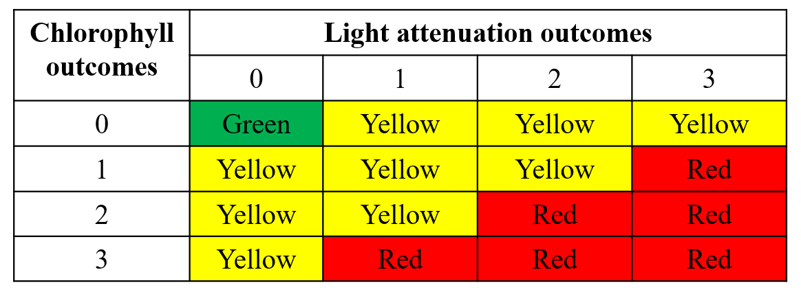
Management action categories assigned to each bay segment and year based on chlorophyll and Secchi depth outcomes.
The results can be viewed with show_matrixpep().
show_matrixpep(dat)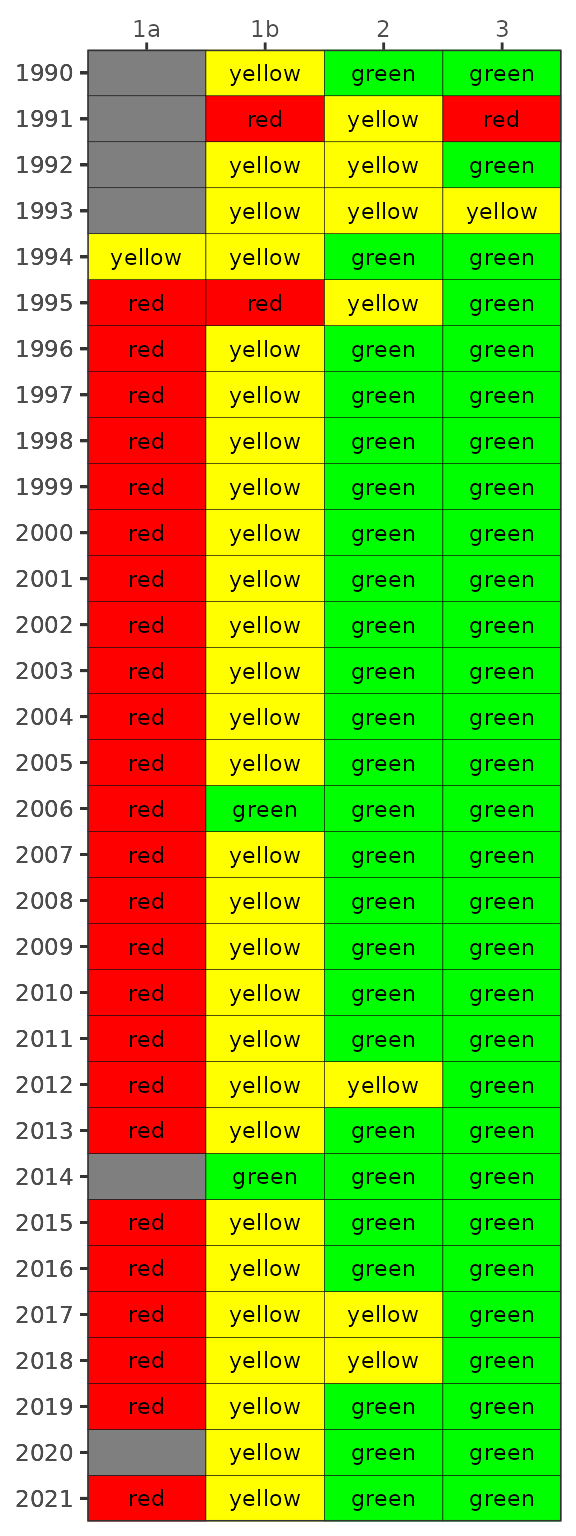
The matrix is also a ggplot object and its layout can be
changed using ggplot elements. Note the use of
txtsz = NULL to remove the color labels.
show_matrixpep(dat, txtsz = NULL) +
  scale_y_continuous(expand = c(0,0), breaks = c(1976:2021)) +
  coord_flip() +
  theme(axis.text.x = element_text(angle = 45, hjust = 1, size = 7))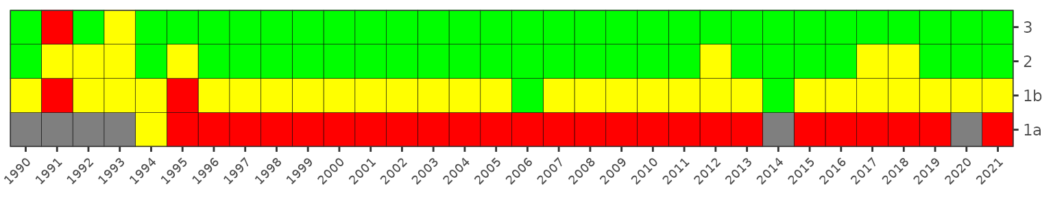
If preferred, the matrix can also be returned in an HTML table that can be sorted and scrolled.
show_matrixpep(dat, asreact = TRUE)Use a sufficiently large number to view the entire matrix.
show_matrixpep(dat, asreact = TRUE, nrows = 200)Bay segment exceedances can also be viewed in a matrix using
show_wqmatrixpep(). The not met/met outcome categories
indicate if the median was above/below the threshold. However, the
small/large exceedances used for the overall report card depend on
degree of overlap of the confidence intervals with the threshold. The
matrix outcome below is a simplification that shows a binary outcome
(not met/met) for location of the median relative to the threshold.
show_wqmatrixpep(dat)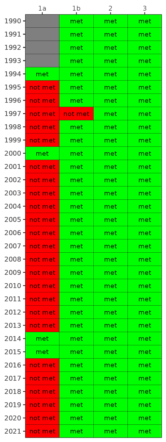
By default, the show_wqmatrixpep() function returns
chlorophyll exceedances by segment. Secchi depth exceedances can be
viewed by changing the param argument. Note that
exceedances are reversed, i.e., lower values are considered less
desirable water quality conditions for Secchi.
show_wqmatrixpep(dat, param = 'sd')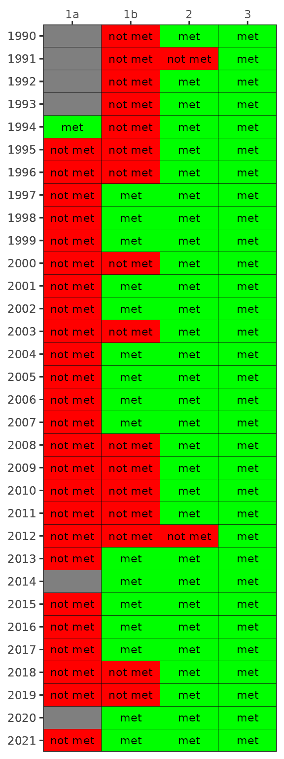
The results from show_matrixpep() for both secchi and
chlorophyll can be combined for an individual segment using the
show_segmatrixpep() function. Only one segment can be
plotted for each function call.
show_segmatrixpep(dat, bay_segment = '1a')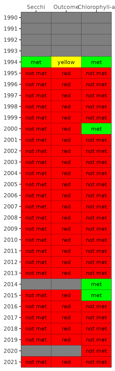
Finally, all plots for a selected segment can be shown together using
the show_plotlypep() function that combines chlorophyll and
secchi data. This function combines outputs from
show_thrpep() and show_segmatrixpep(). The
final plot is interactive and can be zoomed by dragging the mouse
pointer over a section of the plot. Information about each cell or value
can be seen by hovering over a location in the plot.
show_plotlypep(rawdat, bay_segment = '1a')Testing different thresholds
By default, all plotting functions use the peptargets
data frame included with the package, which assigns a threshold of 6.5
ft for secchi depth and 5.5 ug/L for chlorophyll to all segments. All
plotting arguments have an optional argument called trgs
that accepts user-provided thresholds. A new data frame can be passed to
this argument to evaluate different thresholds. The following
demonstrates how to create a custom thresholds data frame (a tibble
specifically) and use it to evaluate changes on reporting outcomes. For
examples, perhaps less stringent thresholds are required for the 1a
segment (lower secchi, higher chlorophyll) and more stringent thresholds
are required for the 3 segment (higher secchi, lower chlorophyll).
segs <- c('1a', '1b', '2', '3')
newtrgs <- data.frame(
  bay_segment = factor(segs, levels = segs),
  name = factor(segs, levels = segs),
  sd_thresh = c(5.0, 5.5, 6.5, 7.5),
  chla_thresh = c(6.5, 6, 5.5, 5),
  stringsAsFactors = F
)
This new data frame can be passed to the plotting functions.
newthr <- show_matrixpep(dat, trgs = newtrgs)
newthr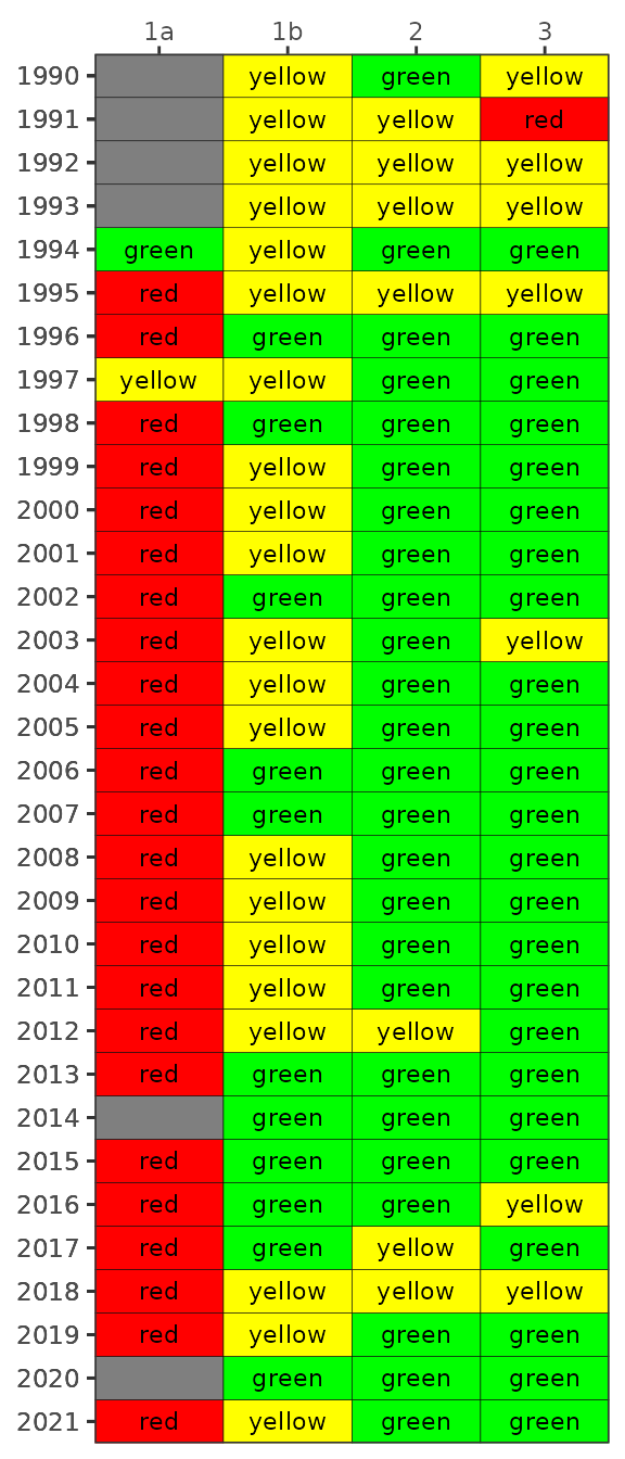
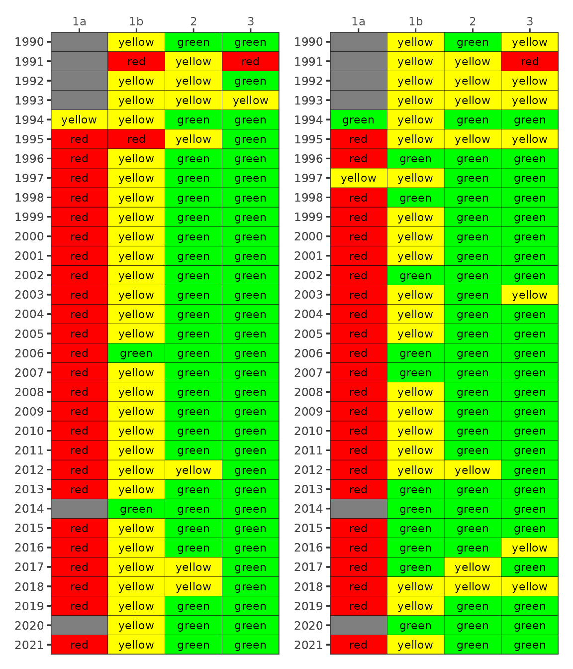
Comparing the default values with the new results can easily be done by plotting the two side by side.
library(patchwork)

oldthr <- show_matrixpep(dat)
oldthr + newthr + plot_layout(ncol = 2)